Code
data(rmb_datasets, package = "rmb")
rmb_datasets$study_design[rmb_datasets$object == "whickham"]
#> [1] "Population-based prospective cohort from Whickham, England, with 20-year mortality follow-up."This article analyzes aggregate Whickham cohort data to illustrate how age confounding can reverse the apparent association between smoking and 20-year mortality—a classic example of Simpson’s paradox described in RMB2e Chapter 3.
The Whickham study was a population-based prospective cohort conducted in a town in northeast England. Women aged 18–64 were interviewed in 1972–1974 and their vital status was ascertained 20 years later. The crude comparison of mortality rates between smokers and non-smokers shows the counterintuitive result that smokers appear to have lower mortality— a finding explained by the younger age distribution of smokers at baseline. Age is a strong confounder because it is associated with both smoking prevalence and 20-year mortality risk (RMB2e Ch. 3).
data(rmb_datasets, package = "rmb")
rmb_datasets$study_design[rmb_datasets$object == "whickham"]
#> [1] "Population-based prospective cohort from Whickham, England, with 20-year mortality follow-up."Is current smoking associated with 20-year all-cause mortality after adjustment for age at baseline?
set.seed(42)
dag <- ggdag::dagify(
  death ~ age + smoke,
  smoke ~ age,
  labels = c(
    death = "20-year mortality",
    smoke = "Current smoking",
    age = "Age at baseline"
  ),
  exposure = "smoke",
  outcome = "death"
)
ggdag::ggdag(dag, use_labels = "label", text = FALSE) +
  ggdag::theme_dag_blank() +
  ggplot2::labs(title = "Whickham: Causal DAG")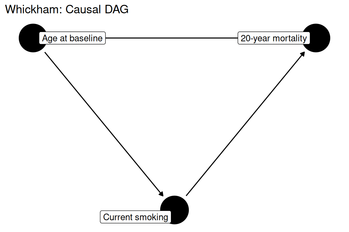
data(whickham, package = "rmb")
dat <- haven::zap_labels(whickham)
dim(dat)
#> [1] 12  4
summary(dat)
#>     vstatus        smoker        agegrp        nn
#>  Min.   :0.0   Min.   :0.0   Min.   :1   Min.   :  7.00
#>  1st Qu.:0.0   1st Qu.:0.0   1st Qu.:1   1st Qu.: 25.75
#>  Median :0.5   Median :0.5   Median :2   Median : 65.00
#>  Mean   :0.5   Mean   :0.5   Mean   :2   Mean   :109.50
#>  3rd Qu.:1.0   3rd Qu.:1.0   3rd Qu.:3   3rd Qu.:165.50
#> Max. :1.0 Max. :1.0 Max. :3 Max. :327.00Because the dataset comprises 12 aggregate rows (age-group × smoking × vital-status counts), the analysis computes stratum-specific mortality rates and odds ratios by age group, then contrasts crude and age-adjusted estimates to illustrate Simpson’s paradox as in RMB2e Chapter 3.
formula_crude <- vstatus ~ smoker
formula_adjusted <- vstatus ~ smoker + agegrp
list(crude = formula_crude, age_adjusted = formula_adjusted)
#> $crude
#> vstatus ~ smoker
#>
#> $age_adjusted
#> vstatus ~ smoker + agegrpdat
#> # A tibble: 12 × 4
#> vstatus smoker agegrp nn
#> <dbl> <dbl> <dbl> <dbl>
#> 1 1 1 1 19
#> 2 0 1 1 269
#> 3 1 0 1 13
#> 4 0 0 1 327
#> 5 1 1 2 78
#> 6 0 1 2 167
#> 7 1 0 2 52
#> 8 0 0 2 147
#> 9 1 1 3 42
#> 10 0 1 3 7
#> 11 1 0 3 165
#> 12 0 0 3 28
with(dat, tapply(nn, list(agegrp, smoker), sum))
#> 0 1
#> 1 340 288
#> 2 199 245
#> 3 193 49mort_by_age <- aggregate(nn ~ agegrp + smoker + vstatus, data = dat, sum)
dead <- subset(mort_by_age, vstatus == 1)
total <- aggregate(nn ~ agegrp + smoker, data = dat, sum)
merged <- merge(dead, total, by = c("agegrp", "smoker"), suffixes = c("_dead", "_total"))
merged$mort_rate <- merged$nn_dead / merged$nn_total
merged$smoker_label <- factor(merged$smoker, levels = c(0, 1), labels = c("Non-smoker", "Smoker"))
ggplot2::ggplot(merged, ggplot2::aes(x = agegrp, y = mort_rate, fill = smoker_label)) +
ggplot2::geom_col(position = "dodge") +
ggplot2::scale_fill_manual(values = c("#1b9e77", "#d95f02")) +
ggplot2::labs(
title = "Mortality rate by age group and smoking status",
x = "Age group",
y = "20-year mortality rate",
fill = NULL
) +
ggplot2::theme_minimal()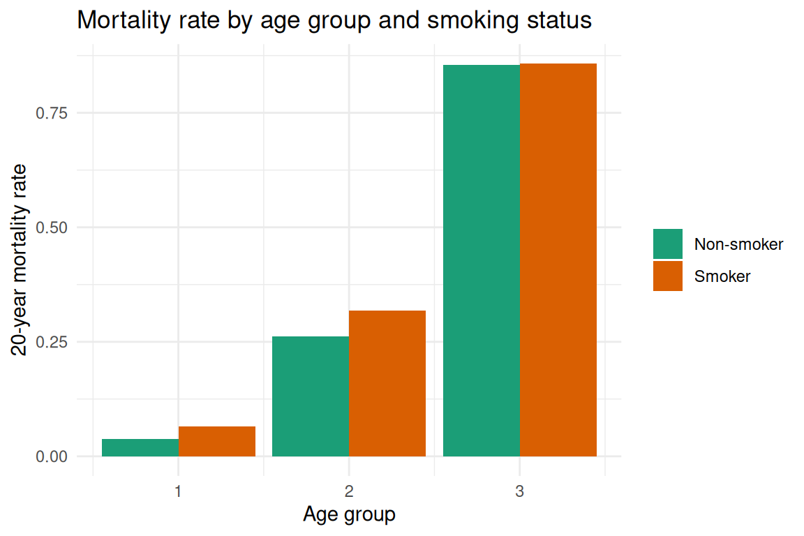
fit_crude <- stats::glm(
  formula_crude,
  data = dat,
  weights = nn,
  family = stats::binomial()
)
fit_adj <- stats::glm(
  formula_adjusted,
  data = dat,
  weights = nn,
  family = stats::binomial()
)
summary(fit_crude)
#>
#> Call:
#> stats::glm(formula = formula_crude, family = stats::binomial(),
#>     data = dat, weights = nn)
#>
#> Coefficients:
#>             Estimate Std. Error z value Pr(>|z|)
#> (Intercept) -0.78052    0.07962  -9.803  < 2e-16 ***
#> smoker      -0.37858    0.12566  -3.013  0.00259 **
#> ---
#> Signif. codes:  0 '***' 0.001 '**' 0.01 '*' 0.05 '.' 0.1 ' ' 1
#>
#> (Dispersion parameter for binomial family taken to be 1)
#>
#>     Null deviance: 1560.3  on 11  degrees of freedom
#> Residual deviance: 1551.1  on 10  degrees of freedom
#> AIC: 1555.1
#>
#> Number of Fisher Scoring iterations: 5
summary(fit_adj)
#>
#> Call:
#> stats::glm(formula = formula_adjusted, family = stats::binomial(),
#>     data = dat, weights = nn)
#>
#> Coefficients:
#>             Estimate Std. Error z value Pr(>|z|)
#> (Intercept)  -5.6708     0.3163  -17.93   <2e-16 ***
#> smoker        0.2212     0.1651    1.34     0.18
#> agegrp        2.4012     0.1348   17.82   <2e-16 ***
#> ---
#> Signif. codes:  0 '***' 0.001 '**' 0.01 '*' 0.05 '.' 0.1 ' ' 1
#>
#> (Dispersion parameter for binomial family taken to be 1)
#>
#>     Null deviance: 1560.32  on 11  degrees of freedom
#> Residual deviance:  991.45  on  9  degrees of freedom
#> AIC: 997.45
#>
#> Number of Fisher Scoring iterations: 6data.frame(
model = c("crude", "age-adjusted"),
AIC = c(stats::AIC(fit_crude), stats::AIC(fit_adj))
)
#> model AIC
#> 1 crude 1555.1167
#> 2 age-adjusted 997.4523or_crude <- exp(stats::coef(fit_crude))
or_adj <- exp(stats::coef(fit_adj))
ci_crude <- exp(stats::confint(fit_crude))
ci_adj <- exp(stats::confint(fit_adj))
data.frame(
model = c("crude smoker OR", "age-adjusted smoker OR"),
odds_ratio = c(unname(or_crude["smoker"]), unname(or_adj["smoker"])),
conf_low = c(ci_crude["smoker", 1], ci_adj["smoker", 1]),
conf_high = c(ci_crude["smoker", 2], ci_adj["smoker", 2])
)
#> model odds_ratio conf_low conf_high
#> 1 crude smoker OR 0.6848366 0.5345661 0.8750872
#> 2 age-adjusted smoker OR 1.2476035 0.9040488 1.7277898The crude analysis shows that smokers have lower or similar mortality to non-smokers, illustrating Simpson’s paradox: smokers are younger on average at baseline, so the negative confounding from age suppresses the harmful effect of smoking. After stratification and age adjustment, the association between smoking and mortality is attenuated or reversed within age groups, consistent with the age-adjusted analysis reported in RMB2e Chapter 3. This example motivates the importance of adjusting for confounders like age before drawing causal conclusions from observational data.