Code
data(rmb_datasets, package = "rmb")
rmb_datasets$study_design[rmb_datasets$object == "esoph"]
#> [1] "Unmatched case-control study of esophageal cancer and alcohol/tobacco exposures in France."This article reproduces the Ille-et-Vilaine esophageal cancer case-control analysis from Tuyns et al. (1977), fitting logistic regression for case status on alcohol, tobacco, and age as in RMB2e Chapter 5.
Esophageal squamous cell carcinoma has historically been associated with heavy alcohol and tobacco use. Tuyns and colleagues (1977) conducted an unmatched case-control study in the Ille-et-Vilaine department of France, recruiting 200 cases and 775 controls to quantify the joint effects of alcohol and tobacco consumption on cancer risk. Because both exposures correlate with age and with each other, confounding-adjusted logistic regression is essential for valid inference (RMB2e Ch. 5).
data(rmb_datasets, package = "rmb")
rmb_datasets$study_design[rmb_datasets$object == "esoph"]
#> [1] "Unmatched case-control study of esophageal cancer and alcohol/tobacco exposures in France."Is heavy alcohol consumption associated with esophageal cancer after adjustment for tobacco use and age group?
set.seed(42)
dag <- ggdag::dagify(
  cancer ~ age + tob + alc,
  alc ~ age,
  tob ~ age,
  labels = c(
    cancer = "Esophageal cancer",
    age = "Age group",
    tob = "Tobacco",
    alc = "Alcohol"
  ),
  exposure = "alc",
  outcome = "cancer"
)
ggdag::ggdag(dag, use_labels = "label", text = FALSE) +
  ggdag::theme_dag_blank() +
  ggplot2::labs(title = "Esoph: Causal DAG")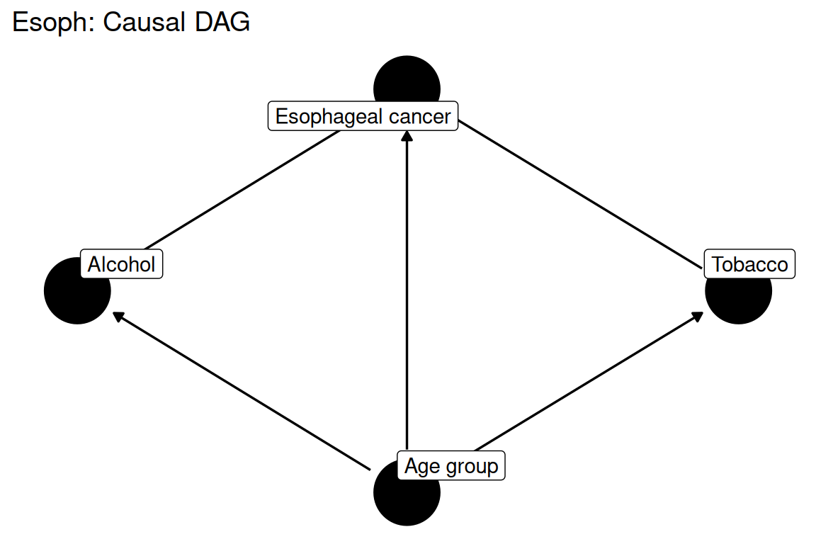
data(esoph, package = "rmb")
dat <- esoph
dim(dat)
#> [1] 975   7
summary(haven::zap_labels(dat[c("case", "age", "agegp", "tob", "tobgp", "alc", "alcgp")]))
#>       case             age            agegp            tob
#>  Min.   :0.0000   Min.   :25.00   Min.   :1.000   Min.   : 0.00
#>  1st Qu.:0.0000   1st Qu.:41.00   1st Qu.:2.000   1st Qu.: 0.00
#>  Median :0.0000   Median :52.00   Median :3.000   Median : 7.50
#>  Mean   :0.2051   Mean   :52.23   Mean   :3.272   Mean   :11.75
#>  3rd Qu.:0.0000   3rd Qu.:63.00   3rd Qu.:4.000   3rd Qu.:17.50
#>  Max.   :1.0000   Max.   :91.00   Max.   :6.000   Max.   :60.00
#>      tobgp            alc             alcgp
#>  Min.   :1.000   Min.   :  0.00   Min.   :1.000
#>  1st Qu.:1.000   1st Qu.: 24.00   1st Qu.:1.000
#>  Median :1.000   Median : 45.00   Median :2.000
#>  Mean   :1.763   Mean   : 52.77   Mean   :1.855
#>  3rd Qu.:2.000   3rd Qu.: 73.00   3rd Qu.:2.000
#> Max. :4.000 Max. :268.00 Max. :4.000Logistic regression models case status on grouped alcohol consumption (alcgp) adjusted for grouped tobacco consumption (tobgp) and age group (agegp), following the categorical-predictor approach in RMB2e Chapter 5.
formula_main <- case ~ alcgp + tobgp + agegp
formula_main
#> case ~ alcgp + tobgp + agegpwith(dat, table(alcgp, case))
#> case
#> alcgp 0 1
#> 1 385 29
#> 2 280 75
#> 3 88 51
#> 4 22 45
with(dat, prop.table(table(alcgp, case), margin = 1))
#> case
#> alcgp 0 1
#> 1 0.92995169 0.07004831
#> 2 0.78873239 0.21126761
#> 3 0.63309353 0.36690647
#> 4 0.32835821 0.67164179
with(dat, table(tobgp, case))
#> case
#> tobgp 0 1
#> 1 448 78
#> 2 178 58
#> 3 98 33
#> 4 51 31alc_rates <- with(dat, tapply(case, alcgp, mean))
alc_df <- data.frame(
alcgp = names(alc_rates),
rate = as.numeric(alc_rates)
)
alc_df$alcgp <- factor(alc_df$alcgp, levels = names(alc_rates))
ggplot2::ggplot(alc_df, ggplot2::aes(x = alcgp, y = rate)) +
ggplot2::geom_col(fill = "#d95f02") +
ggplot2::labs(
title = "Crude case rate by alcohol consumption group",
x = "Alcohol group (gm/day)",
y = "Proportion cases"
) +
ggplot2::theme_minimal()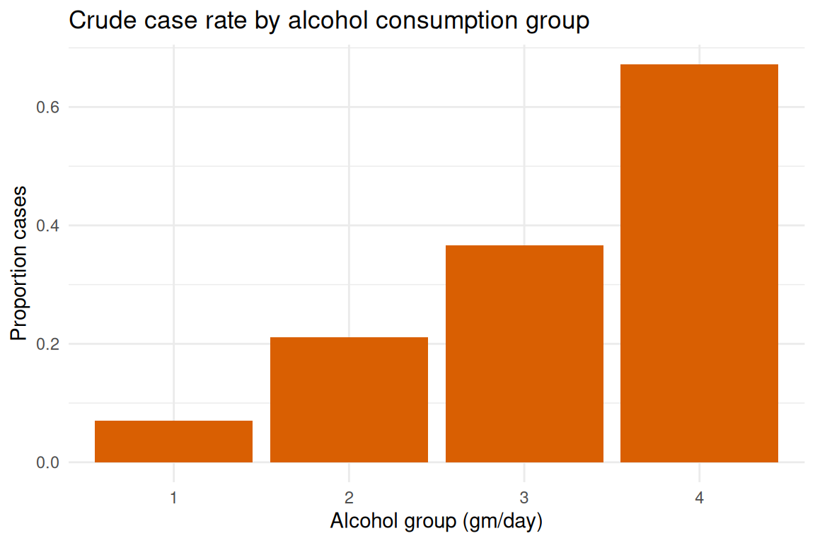
fit <- stats::glm(formula_main, data = dat, family = stats::binomial())
summary(fit)
#>
#> Call:
#> stats::glm(formula = formula_main, family = stats::binomial(),
#>     data = dat)
#>
#> Coefficients:
#>             Estimate Std. Error z value Pr(>|z|)
#> (Intercept) -7.16053    0.50912 -14.065  < 2e-16 ***
#> alcgp        1.09868    0.10303  10.664  < 2e-16 ***
#> tobgp        0.43357    0.09384   4.620 3.83e-06 ***
#> agegp        0.74321    0.08178   9.088  < 2e-16 ***
#> ---
#> Signif. codes:  0 '***' 0.001 '**' 0.01 '*' 0.05 '.' 0.1 ' ' 1
#>
#> (Dispersion parameter for binomial family taken to be 1)
#>
#>     Null deviance: 989.49  on 974  degrees of freedom
#> Residual deviance: 730.95  on 971  degrees of freedom
#> AIC: 738.95
#>
#> Number of Fisher Scoring iterations: 5fit_alc_only <- stats::glm(case ~ alcgp, data = dat, family = stats::binomial())
stats::anova(fit_alc_only, fit, test = "Chisq")
#> Analysis of Deviance Table
#>
#> Model 1: case ~ alcgp
#> Model 2: case ~ alcgp + tobgp + agegp
#> Resid. Df Resid. Dev Df Deviance Pr(>Chi)
#> 1 973 845.72
#> 2 971 730.95 2 114.77 < 2.2e-16 ***
#> ---
#> Signif. codes: 0 '***' 0.001 '**' 0.01 '*' 0.05 '.' 0.1 ' ' 1or <- exp(stats::coef(fit))
ci <- exp(stats::confint(fit))
data.frame(
term = names(or),
odds_ratio = unname(or),
conf_low = ci[, 1],
conf_high = ci[, 2],
p_value = summary(fit)$coefficients[, "Pr(>|z|)"]
)
#> term odds_ratio conf_low conf_high p_value
#> (Intercept) (Intercept) 0.0007766439 0.0002745303 0.002025383 6.270979e-45
#> alcgp alcgp 3.0002047835 2.4619572608 3.689197049 1.497794e-26
#> tobgp tobgp 1.5427575820 1.2840941386 1.856194529 3.831928e-06
#> agegp agegp 2.1026764394 1.7986710045 2.479600792 1.006057e-19Heavy alcohol consumption is strongly associated with esophageal cancer risk after adjustment for tobacco use and age, consistent with the dose-response pattern reported by Tuyns et al. (1977) and discussed in RMB2e Chapter 5. Tobacco consumption and older age are independently associated with elevated odds. The likelihood-ratio test comparing the alcohol-only model to the full model confirms that tobacco and age explain additional variation in case status beyond alcohol alone. These findings underscore the importance of mutual adjustment when exposures are correlated.