Code
data(rmb_datasets, package = "rmb")
rmb_datasets$study_design[rmb_datasets$object == "mira_hsv"]
#> [1] "Randomized trial evaluating diaphragm-based HIV prevention with repeated HSV-2 follow-up."This article applies logistic regression to the MIRA HSV-2 dataset, assessing whether having a new sexual partner is associated with incident HSV-2 infection after adjustment for age and STI history (RMB2e Chapter 5).
Herpes simplex virus type 2 (HSV-2) is the leading cause of genital ulcer disease worldwide and an important HIV cofactor. The MIRA trial evaluated diaphragm-based HIV prevention in sub-Saharan Africa; a secondary analysis by de Bruyn et al. (2011) examined predictors of incident HSV-2 among participants. Acquiring a new sexual partner substantially increases exposure risk, but age and prior STI history confound this relationship because older women and those with STI history are more likely to have established partners and different HSV-2 susceptibility (RMB2e Ch. 5).
data(rmb_datasets, package = "rmb")
rmb_datasets$study_design[rmb_datasets$object == "mira_hsv"]
#> [1] "Randomized trial evaluating diaphragm-based HIV prevention with repeated HSV-2 follow-up."Is having a new sexual partner associated with incident HSV-2 infection after adjustment for age category and prior STI history?
set.seed(42)
dag <- ggdag::dagify(
  hsv2 ~ newpart + sti + age,
  newpart ~ age,
  labels = c(
    hsv2 = "Incident HSV-2",
    newpart = "New partner",
    sti = "STI history",
    age = "Age category"
  ),
  exposure = "newpart",
  outcome = "hsv2"
)
ggdag::ggdag(dag, use_labels = "label", text = FALSE) +
  ggdag::theme_dag_blank() +
  ggplot2::labs(title = "MIRA: Causal DAG")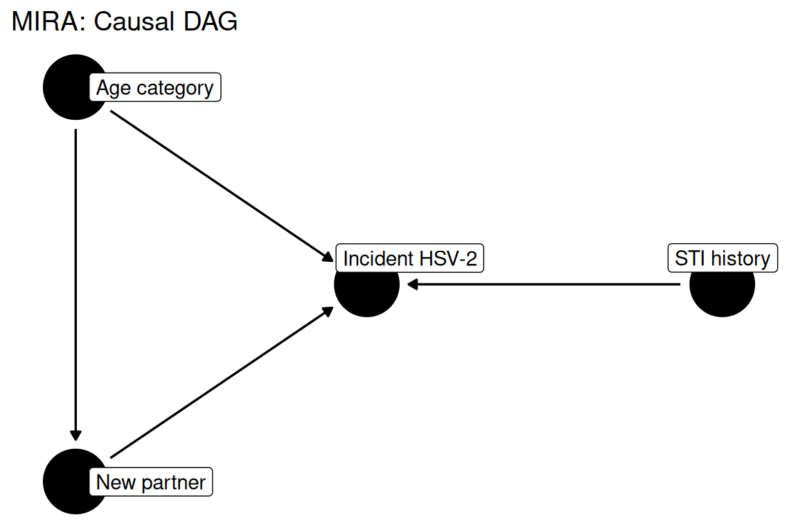
data(mira_hsv, package = "rmb")
dat <- mira_hsv
dim(dat)
#> [1] 6069    6
summary(haven::zap_labels(dat[c("hsv2", "newparts", "stihx", "agecat")]))
#>       hsv2            newparts          stihx             agecat
#>  Min.   :0.00000   Min.   :0.0000   Min.   :0.00000   Min.   :1.000
#>  1st Qu.:0.00000   1st Qu.:0.0000   1st Qu.:0.00000   1st Qu.:1.000
#>  Median :0.00000   Median :0.0000   Median :0.00000   Median :1.000
#>  Mean   :0.01714   Mean   :0.1234   Mean   :0.09738   Mean   :1.588
#>  3rd Qu.:0.00000   3rd Qu.:0.0000   3rd Qu.:0.00000   3rd Qu.:2.000
#> Max. :1.00000 Max. :1.0000 Max. :1.00000 Max. :3.000Logistic regression models incident HSV-2 as a function of new partner status, prior STI history, and age category, following the categorical-predictor approach in RMB2e Chapter 5.
formula_main <- hsv2 ~ newparts + stihx + agecat
formula_main
#> hsv2 ~ newparts + stihx + agecathsv_rates <- with(dat, tapply(hsv2, list(agecat, newparts), mean, na.rm = TRUE))
hsv_df <- as.data.frame(as.table(hsv_rates))
names(hsv_df) <- c("agecat", "newparts", "rate")
ggplot2::ggplot(hsv_df, ggplot2::aes(x = agecat, y = rate, fill = newparts)) +
ggplot2::geom_col(position = "dodge") +
ggplot2::scale_fill_manual(
values = c("#1b9e77", "#d95f02"),
labels = c("No new partner", "New partner")
) +
ggplot2::labs(
title = "MIRA: HSV-2 incidence by age and new partner",
x = "Age category",
y = "HSV-2 incidence proportion",
fill = NULL
) +
ggplot2::theme_minimal()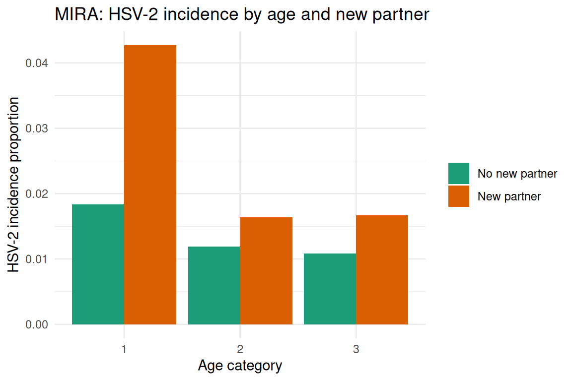
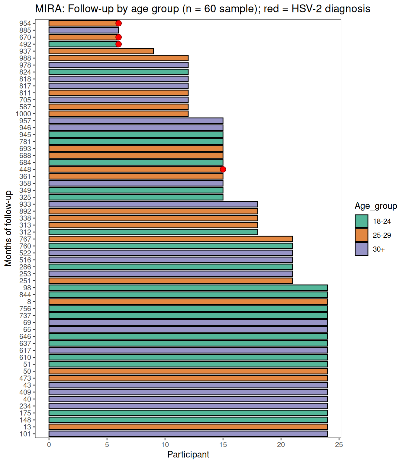
The swimmer plot shows follow-up timelines for a stratified random sample of 60 participants (20 per age group), with red dots indicating months of HSV-2 diagnosis.
set.seed(42)
dat_full <- as.data.frame(dat)
first_visit <- dat_full[!duplicated(dat_full$id), c("id", "agecat")]
ids_sub <- unlist(
  tapply(
    first_visit$id, first_visit$agecat,
    function(x) sample(x, min(20L, length(x)))
  )
)
dat_sub <- dat_full[dat_full$id %in% ids_sub, ]

# Summarize to one row per subject (end = last observed month)
dat_ends <- aggregate(mos ~ id, data = dat_sub, FUN = max)
names(dat_ends)[2] <- "end"
dat_sum <- merge(dat_ends, first_visit, by = "id")
dat_sum$Age_group <- factor(
  dat_sum$agecat,
  levels = c(1, 2, 3),
  labels = c("18-24", "25-29", "30+")
)
dat_events <- dat_sub[dat_sub$hsv2 == 1, ]

swimplot::swimmer_plot(
  df = dat_sum, id = "id", end = "end",
  name_fill = "Age_group", increasing = FALSE,
  col = "black", alpha = 0.75, width = 0.8
) +
  swimplot::swimmer_points(
    df = dat_events, id = "id", time = "mos",
    shape = 21, size = 3, col = "darkred", fill = "red"
  ) +
  ggplot2::scale_fill_manual(
    values = c("#1b9e77", "#d95f02", "#7570b3")
  ) +
  ggplot2::labs(
    x = "Months of follow-up",
    y = "Participant",
    title = "MIRA: Follow-up by age group (n = 60 sample); red = HSV-2 diagnosis"
  )
fit <- stats::glm(formula_main, data = dat, family = stats::binomial())
summary(fit)
#>
#> Call:
#> stats::glm(formula = formula_main, family = stats::binomial(),
#>     data = dat)
#>
#> Coefficients:
#>             Estimate Std. Error z value Pr(>|z|)
#> (Intercept)  -3.6653     0.2718 -13.485  < 2e-16 ***
#> newparts      0.6654     0.2388   2.787  0.00532 **
#> stihx         0.6821     0.2557   2.667  0.00765 **
#> agecat       -0.3955     0.1679  -2.355  0.01850 *
#> ---
#> Signif. codes:  0 '***' 0.001 '**' 0.01 '*' 0.05 '.' 0.1 ' ' 1
#>
#> (Dispersion parameter for binomial family taken to be 1)
#>
#>     Null deviance: 1052.1  on 6068  degrees of freedom
#> Residual deviance: 1029.7  on 6065  degrees of freedom
#> AIC: 1037.7
#>
#> Number of Fisher Scoring iterations: 7fit_unadj <- stats::glm(hsv2 ~ newparts, data = dat, family = stats::binomial())
stats::anova(fit_unadj, fit, test = "Chisq")
#> Analysis of Deviance Table
#>
#> Model 1: hsv2 ~ newparts
#> Model 2: hsv2 ~ newparts + stihx + agecat
#> Resid. Df Resid. Dev Df Deviance Pr(>Chi)
#> 1 6067 1042.7
#> 2 6065 1029.7 2 13.014 0.001493 **
#> ---
#> Signif. codes: 0 '***' 0.001 '**' 0.01 '*' 0.05 '.' 0.1 ' ' 1or <- exp(stats::coef(fit))
ci <- exp(stats::confint(fit))
data.frame(
term = names(or),
odds_ratio = unname(or),
conf_low = ci[, 1],
conf_high = ci[, 2],
p_value = summary(fit)$coefficients[, "Pr(>|z|)"]
)
#> term odds_ratio conf_low conf_high p_value
#> (Intercept) (Intercept) 0.0255975 0.01495537 0.04348408 1.907393e-41
#> newparts newparts 1.9453339 1.19407446 3.05704622 5.320205e-03
#> stihx stihx 1.9779842 1.16746089 3.19799069 7.650349e-03
#> agecat agecat 0.6733654 0.47858444 0.92591954 1.849780e-02New partner acquisition is associated with increased odds of incident HSV-2 after adjustment for age and STI history, consistent with the transmission dynamics of a sexually transmitted pathogen and the findings of de Bruyn et al. (2011). Prior STI history is a marker of sexual network exposure and susceptibility, while age reflects accumulated exposure and possible partial immunity. This analysis illustrates how logistic regression for binary outcomes adjusts for multiple categorical confounders simultaneously, a core application in RMB2e Chapter 5.