Code
data(rmb_datasets, package = "rmb")
rmb_datasets$study_design[rmb_datasets$object == "hers_nodm_longitudinal"]
#> [1] "Longitudinal repeated-measures HERS subset restricted to participants without diabetes."This article models longitudinal systolic blood pressure trajectories in HERS participants without diabetes, examining whether HRT assignment and exercise interact to affect blood pressure over follow-up visits (RMB2e Chapter 11).
Hormone therapy and lifestyle behaviors such as exercise may jointly influence cardiovascular risk factors in postmenopausal women. The HERS longitudinal dataset provides repeated measurements of systolic blood pressure over multiple visits, enabling examination of within-subject trajectories and potential treatment–lifestyle interactions. RMB2e Chapter 11 uses this structure to illustrate repeated-measures regression and missing-data approaches.
data(rmb_datasets, package = "rmb")
rmb_datasets$study_design[rmb_datasets$object == "hers_nodm_longitudinal"]
#> [1] "Longitudinal repeated-measures HERS subset restricted to participants without diabetes."We ask: does regular exercise moderate the association between HRT assignment and longitudinal systolic blood pressure in postmenopausal women without diabetes?
set.seed(42)
dag <- ggdag::dagify(
  sbp ~ hrt + exercise + int_hrt_exercise + bmi + age,
  int_hrt_exercise ~ hrt + exercise,
  labels = c(
    sbp = "Systolic BP",
    hrt = "HRT assignment",
    exercise = "Exercise",
    int_hrt_exercise = "HRT x exercise",
    bmi = "BMI",
    age = "Age"
  ),
  exposure = "hrt",
  outcome = "sbp"
)
ggdag::ggdag(dag, use_labels = "label", text = FALSE) +
  ggdag::theme_dag_blank() +
  ggplot2::labs(title = "HERS longitudinal: Causal DAG")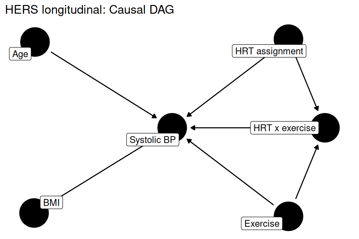
data(hers_nodm_longitudinal, package = "rmb")
dat <- hers_nodm_longitudinal
dim(dat)
#> [1] 9217   15
summary(haven::zap_labels(dat[c("sbp", "group", "exercise", "bmi", "age", "visit")]))
#>       sbp            group           exercise           bmi
#>  Min.   : 81.0   Min.   :0.0000   Min.   :0.0000   Min.   :14.73
#>  1st Qu.:121.0   1st Qu.:0.0000   1st Qu.:0.0000   1st Qu.:24.08
#>  Median :132.0   Median :0.0000   Median :0.0000   Median :26.96
#>  Mean   :134.2   Mean   :0.4917   Mean   :0.3716   Mean   :27.69
#>  3rd Qu.:146.0   3rd Qu.:1.0000   3rd Qu.:1.0000   3rd Qu.:30.43
#>  Max.   :228.0   Max.   :1.0000   Max.   :1.0000   Max.   :57.56
#>                                   NAs    :79       NAs    :45
#>       age            visit
#>  Min.   :44.00   Min.   :0.000
#>  1st Qu.:62.00   1st Qu.:1.000
#>  Median :67.00   Median :2.000
#>  Mean   :66.68   Mean   :1.925
#>  3rd Qu.:72.00   3rd Qu.:3.000
#>  Max.   :79.00   Max.   :5.000
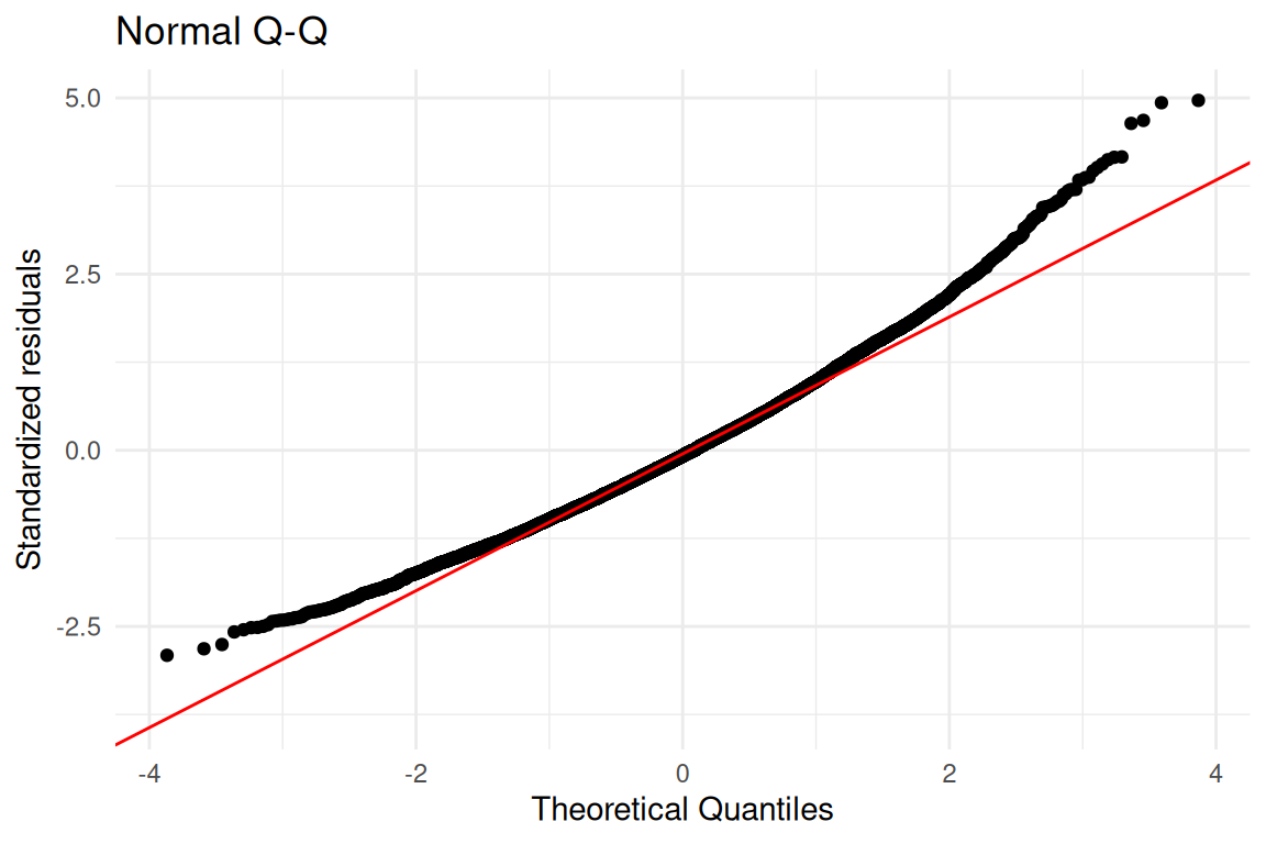
#> We fit a linear regression model for systolic blood pressure with an HRT-by-exercise interaction term, adjusting for BMI, age, smoking, and visit number. The model ignores within-person correlation but illustrates the interaction parameterization discussed in RMB2e Chapter 11.
formula_sbp <- sbp ~ group * exercise + bmi + age + csmker + visit
formula_sbp
#> sbp ~ group * exercise + bmi + age + csmker + visitdat$group_exercise <- interaction(dat$group, dat$exercise)
dat$group_exercise_label <- factor(
dat$group_exercise,
labels = c("Pbo/No ex", "HRT/No ex", "Pbo/Ex", "HRT/Ex")
)
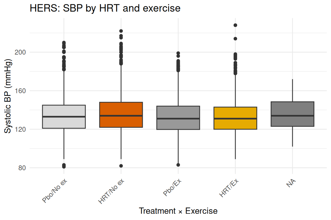
ggplot2::ggplot(dat, ggplot2::aes(x = group_exercise_label, y = sbp, fill = group_exercise_label)) +
ggplot2::geom_boxplot() +
ggplot2::scale_fill_manual(values = c("grey85", "#d95f02", "grey60", "#e6ab02")) +
ggplot2::labs(
title = "HERS: SBP by HRT and exercise",
x = "Treatment × Exercise",
y = "Systolic BP (mmHg)"
) +
ggplot2::theme_minimal() +
ggplot2::theme(
legend.position = "none",
axis.text.x = ggplot2::element_text(angle = 45, hjust = 1)
)
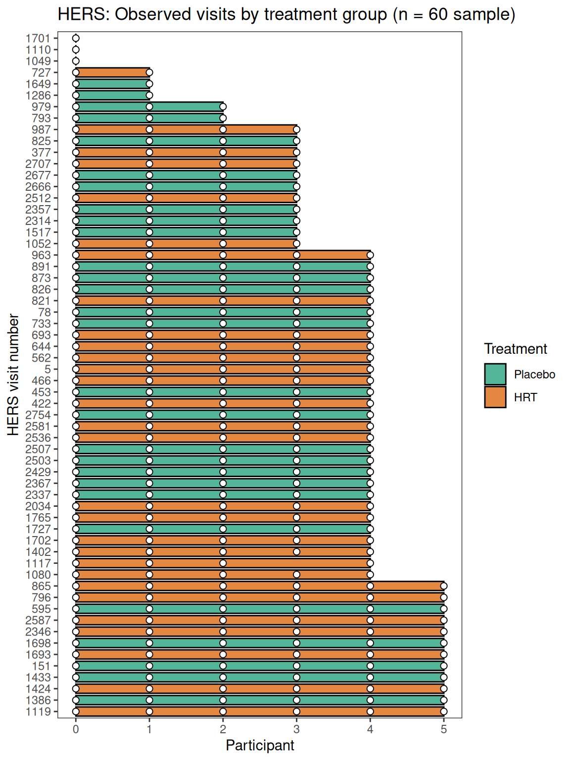
The swimmer plot shows visit attendance for a stratified random sample of 60 participants (30 per treatment arm), with a dot at each completed visit.
set.seed(42)
dat_full <- as.data.frame(dat)
first_obs <- dat_full[!duplicated(dat_full$pptid), c("pptid", "group")]
ids_0 <- sample(first_obs$pptid[first_obs$group == 0], 30)
ids_1 <- sample(first_obs$pptid[first_obs$group == 1], 30)
dat_sub <- dat_full[dat_full$pptid %in% c(ids_0, ids_1), ]

dat_ends <- aggregate(visit ~ pptid, data = dat_sub, FUN = max)
names(dat_ends)[2] <- "last_visit"
dat_sum <- merge(
  dat_ends,
  first_obs[first_obs$pptid %in% c(ids_0, ids_1), ],
  by = "pptid"
)
dat_sum$Treatment <- factor(
  dat_sum$group,
  levels = c(0, 1),
  labels = c("Placebo", "HRT")
)

swimplot::swimmer_plot(
  df = dat_sum, id = "pptid", end = "last_visit",
  name_fill = "Treatment", increasing = FALSE,
  col = "black", alpha = 0.75, width = 0.8
) +
  swimplot::swimmer_points(
    df = dat_sub, id = "pptid", time = "visit",
    shape = 21, size = 2, col = "black", fill = "white"
  ) +
  ggplot2::scale_fill_manual(values = c("#1b9e77", "#d95f02")) +
  ggplot2::labs(
    x = "HERS visit number",
    y = "Participant",
    title = "HERS: Observed visits by treatment group (n = 60 sample)"
  )
fit_sbp <- stats::lm(formula_sbp, data = dat)
summary(fit_sbp)
#>
#> Call:
#> stats::lm(formula = formula_sbp, data = dat)
#>
#> Residuals:
#>     Min      1Q  Median      3Q     Max
#> -53.712 -13.021  -1.456  11.161  91.647
#>
#> Coefficients:
#>                Estimate Std. Error t value Pr(>|t|)
#> (Intercept)    90.45811    2.56495  35.267  < 2e-16 ***
#> group           2.17496    0.48933   4.445 8.90e-06 ***
#> exercise       -1.13786    0.56817  -2.003 0.045243 *
#> bmi             0.26378    0.03840   6.869 6.89e-12 ***
#> age             0.52541    0.03035  17.313  < 2e-16 ***
#> csmker          0.96775    0.56667   1.708 0.087713 .
#> visit           0.45587    0.13311   3.425 0.000618 ***
#> group:exercise -1.60051    0.80192  -1.996 0.045981 *
#> ---
#> Signif. codes:  0 '***' 0.001 '**' 0.01 '*' 0.05 '.' 0.1 ' ' 1
#>
#> Residual standard error: 18.47 on 9083 degrees of freedom
#>   (126 observations deleted due to missingness)
#> Multiple R-squared:  0.04008,    Adjusted R-squared:  0.03934
#> F-statistic: 54.18 on 7 and 9083 DF, p-value: < 2.2e-16fit_data <- data.frame(
fitted = stats::fitted(fit_sbp),
residuals = stats::residuals(fit_sbp),
std_residuals = stats::rstandard(fit_sbp)
)
ggplot2::ggplot(fit_data, ggplot2::aes(x = fitted, y = residuals)) +
ggplot2::geom_point(alpha = 0.25, size = 0.5) +
ggplot2::geom_hline(yintercept = 0, linetype = "dashed", color = "red") +
ggplot2::geom_smooth(se = FALSE, color = "blue") +
ggplot2::labs(
title = "Residuals vs Fitted",
x = "Fitted values",
y = "Residuals"
) +
ggplot2::theme_minimal()
ggplot2::ggplot(fit_data, ggplot2::aes(sample = std_residuals)) +
ggplot2::stat_qq() +
ggplot2::stat_qq_line(color = "red") +
ggplot2::labs(
title = "Normal Q-Q",
x = "Theoretical Quantiles",
y = "Standardized residuals"
) +
ggplot2::theme_minimal()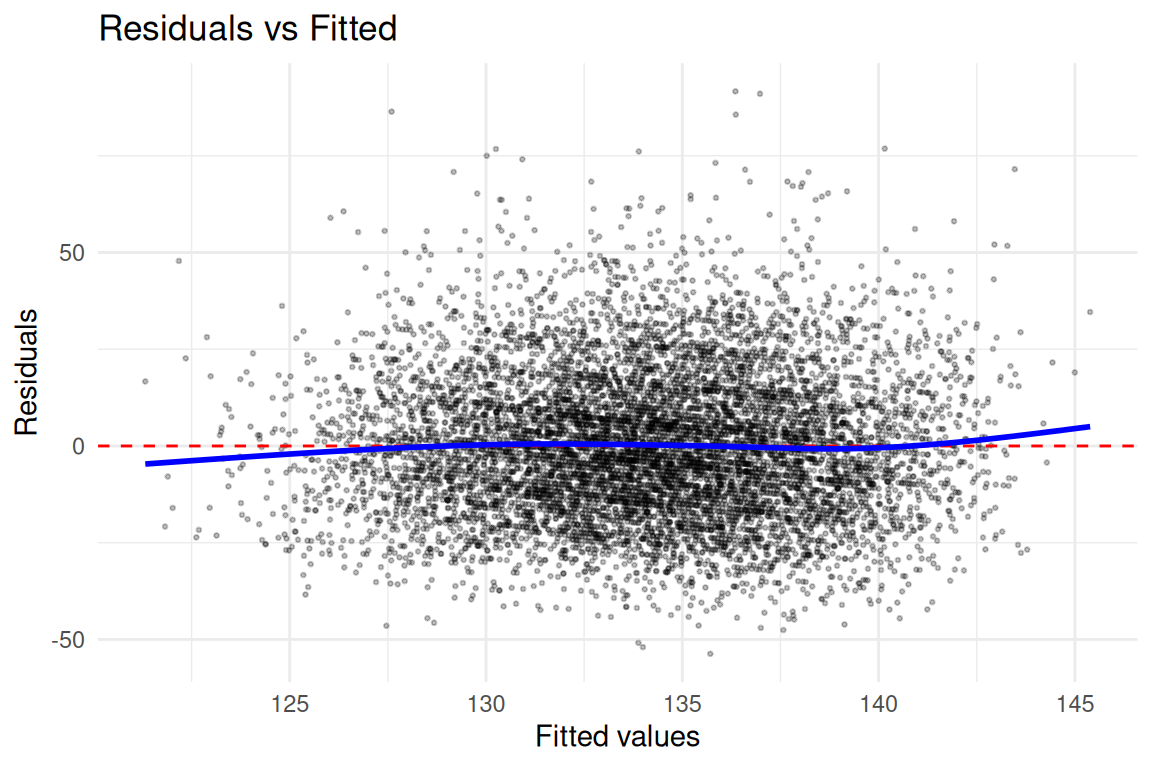
ci <- stats::confint(fit_sbp)
coef_tab <- data.frame(
  term = names(stats::coef(fit_sbp)),
  estimate = stats::coef(fit_sbp),
  conf_low = ci[, 1],
  conf_high = ci[, 2],
  p_value = summary(fit_sbp)$coefficients[, "Pr(>|t|)"]
)
coef_tab
#>                          term   estimate   conf_low   conf_high       p_value
#> (Intercept)       (Intercept) 90.4581066 85.4302297 95.48598350 1.828260e-255
#> group                   group  2.1749590  1.2157550  3.13416313  8.904358e-06
#> exercise             exercise -1.1378570 -2.2516014 -0.02411253  4.524303e-02
#> bmi                       bmi  0.2637767  0.1885017  0.33905175  6.891714e-12
#> age                       age  0.5254143  0.4659260  0.58490251  4.276484e-66
#> csmker                 csmker  0.9677497 -0.1430581  2.07855756  8.771269e-02
#> visit                   visit  0.4558707  0.1949420  0.71679940  6.181419e-04
#> group:exercise group:exercise -1.6005099 -3.1724596 -0.02856013 4.598118e-02The interaction between HRT assignment and exercise on systolic blood pressure examines whether lifestyle behaviors modify the cardiovascular effects of hormone therapy. As discussed in RMB2e Chapter 11, the longitudinal structure of HERS requires accounting for within-person correlation; the regression model presented here is an approximation useful for illustrating interaction parameterization, while a proper generalized estimating equations (GEE) or mixed-effects model would be needed for valid inference accounting for repeated measures.