Code
data(rmb_datasets, package = "rmb")
rmb_datasets$study_design[rmb_datasets$object == "mros"]
#> [1] "Prospective cohort of older men in the Osteoporotic Fractures in Men (MrOS) study."This article fits a Cox proportional hazards model to the MrOS dataset, evaluating whether lower bone mineral density quantiles predict higher event hazard in older men after adjustment for body weight.
The Osteoporotic Fractures in Men (MrOS) study enrolled community-dwelling men aged 65 years and older at six US clinical sites beginning in 2000 (Orwoll et al. 2005). Low bone mineral density (BMD) is a well-established predictor of fracture and mortality risk in older men, though body weight is a strong confounder because heavier men tend to have higher BMD and independently different event rates. This survival analysis applies the Cox proportional hazards framework described in RMB2e Chapter 6.
data(rmb_datasets, package = "rmb")
rmb_datasets$study_design[rmb_datasets$object == "mros"]
#> [1] "Prospective cohort of older men in the Osteoporotic Fractures in Men (MrOS) study."Are lower bone mineral density quantiles associated with higher event hazard after adjustment for body weight in older men?
set.seed(42)
dag <- ggdag::dagify(
  surv ~ bmd + weight,
  bmd ~ weight,
  labels = c(
    surv = "Event/death",
    bmd = "BMD quantile",
    weight = "Body weight"
  ),
  exposure = "bmd",
  outcome = "surv"
)
ggdag::ggdag(dag, use_labels = "label", text = FALSE) +
  ggdag::theme_dag_blank() +
  ggplot2::labs(title = "MrOS: Causal DAG")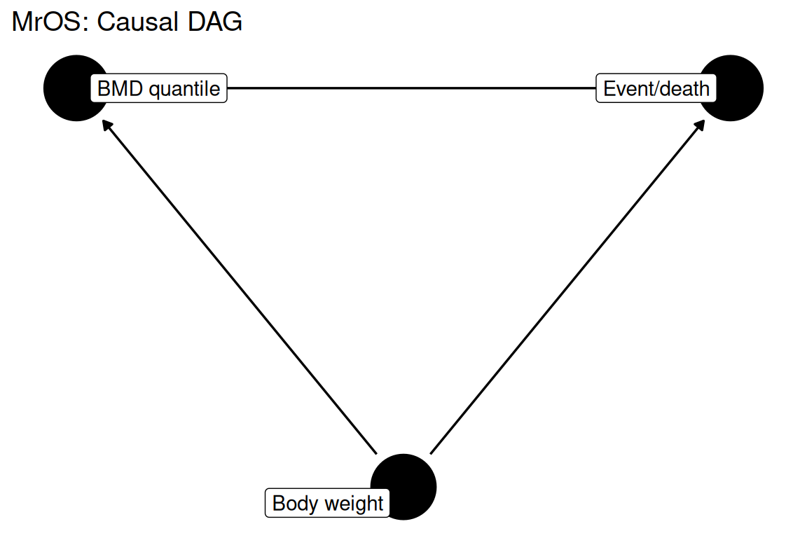
data(mros, package = "rmb")
dat <- mros
dim(dat)
#> [1] 5994    5
summary(haven::zap_labels(dat[c("bmd3", "months", "years", "status", "weight")]))
#>       bmd3           months         years           status
#>  Min.   :1.000   Min.   : 0.0   Min.   :0.000   Min.   :0.0000
#>  1st Qu.:1.000   1st Qu.:60.0   1st Qu.:4.887   1st Qu.:0.0000
#>  Median :2.000   Median :66.0   Median :5.369   Median :0.0000
#>  Mean   :2.008   Mean   :62.4   Mean   :5.086   Mean   :0.3078
#>  3rd Qu.:3.000   3rd Qu.:73.0   3rd Qu.:5.960   3rd Qu.:0.0000
#>  Max.   :3.000   Max.   :85.0   Max.   :6.946   Max.   :2.0000
#>      weight
#>  Min.   : 48.50
#>  1st Qu.: 73.70
#>  Median : 81.80
#>  Mean   : 83.15
#>  3rd Qu.: 91.00
#> Max. :144.10A Cox proportional hazards model is fitted with bmd3 (three quantiles of BMD, coded as factor) and body weight as predictors, using follow-up time in years as the time scale (RMB2e Ch. 6 / Orwoll 2005).
with(dat, table(bmd3, status))
#>     status
#> bmd3    0    1    2
#>    1 1440  287  238
#>    2 1653  134  230
#>    3 1713  110  189
with(dat, tapply(years, bmd3, summary))
#> $`1`
#>    Min. 1st Qu.  Median    Mean 3rd Qu.    Max.
#>   0.000   4.715   5.273   4.882   5.908   6.749
#>
#> $`2`
#>    Min. 1st Qu.  Median    Mean 3rd Qu.    Max.
#> 0.01095 4.92539 5.38535 5.15285 5.96030 6.75702
#>
#> $`3`
#>    Min. 1st Qu.  Median    Mean 3rd Qu.    Max.
#> 0.01095 4.96372 5.42094 5.21683 5.98494 6.94593
with(dat, tapply(weight, bmd3, mean))
#>        1        2        3
#> 77.11654 83.10759 89.09051dat$bmd3_plot <- factor(
dat$bmd3,
labels = c("BMD Q1 (low)", "BMD Q2", "BMD Q3 (high)")
)
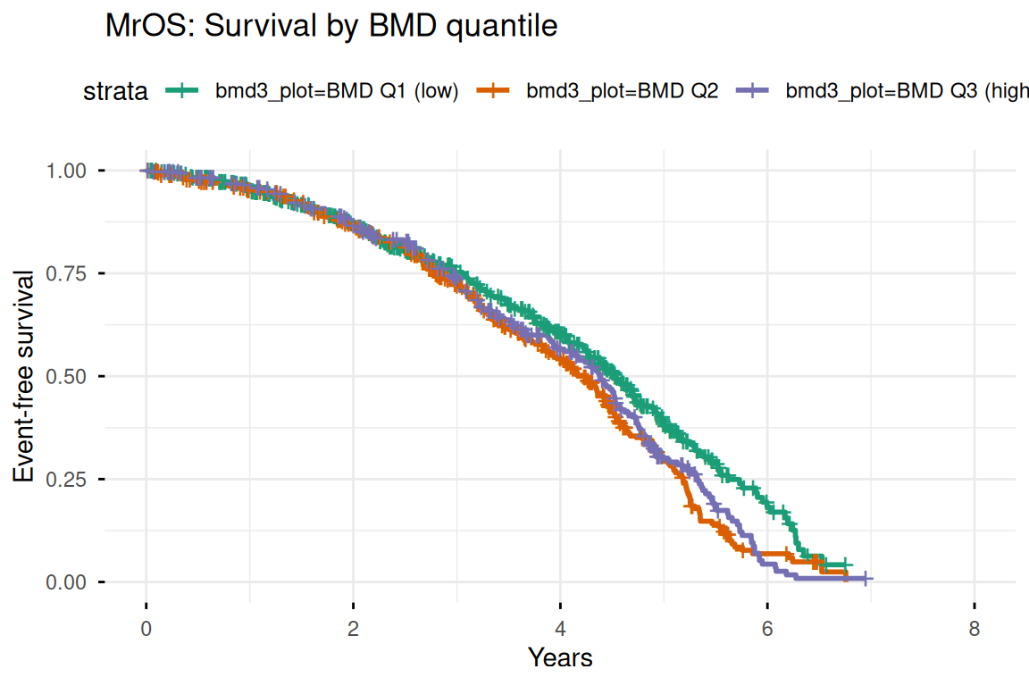
km_fit <- survival::survfit(survival::Surv(years, status) ~ bmd3_plot, data = dat)
survminer::ggsurvplot(
km_fit,
data = dat,
title = "MrOS: Survival by BMD quantile",
xlab = "Years",
ylab = "Event-free survival",
legend.title = NULL,
ggtheme = ggplot2::theme_minimal(),
palette = c("#1b9e77", "#d95f02", "#7570b3"),
conf.int = FALSE,
censor = TRUE
)
fit <- survival::coxph(formula_main, data = dat, ties = "breslow")
summary(fit)
#> Call:
#> survival::coxph(formula = formula_main, data = dat, ties = "breslow")
#>
#>   n= 1188, number of events= 657
#>    (4806 observations deleted due to missingness)
#>
#>                    coef exp(coef)  se(coef)      z Pr(>|z|)
#> factor(bmd3)2  0.298690  1.348092  0.093916  3.180  0.00147 **
#> factor(bmd3)3  0.289976  1.336396  0.104930  2.764  0.00572 **
#> weight        -0.005219  0.994795  0.003081 -1.694  0.09032 .
#> ---
#> Signif. codes:  0 '***' 0.001 '**' 0.01 '*' 0.05 '.' 0.1 ' ' 1
#>
#>               exp(coef) exp(-coef) lower .95 upper .95
#> factor(bmd3)2    1.3481     0.7418    1.1214     1.621
#> factor(bmd3)3    1.3364     0.7483    1.0880     1.642
#> weight           0.9948     1.0052    0.9888     1.001
#>
#> Concordance= 0.527  (se = 0.013 )
#> Likelihood ratio test= 12.78  on 3 df,   p=0.005
#> Wald test            = 12.62  on 3 df,   p=0.006
#> Score (logrank) test = 12.66 on 3 df, p=0.005ph_test <- survival::cox.zph(fit)
ph_test
#> chisq df p
#> factor(bmd3) 5.1042 2 0.078
#> weight 0.0127 1 0.910
#> GLOBAL 5.7592 3 0.124| term | hazard_ratio | conf_low | conf_high | p_value | |
|---|---|---|---|---|---|
| factor(bmd3)2 | factor(bmd3)2 | 1.348 | 1.121 | 1.621 | 0.001 |
| factor(bmd3)3 | factor(bmd3)3 | 1.336 | 1.088 | 1.642 | 0.006 |
| weight | weight | 0.995 | 0.989 | 1.001 | 0.090 |
Men in lower BMD quantiles have higher hazard of the composite event after adjustment for body weight, consistent with the dose-response relationship between bone density and fracture/mortality risk described in RMB2e Chapter 6. Weight is also independently predictive, reflecting the complex relationship between adiposity and skeletal outcomes in older men. These findings illustrate how Cox regression can simultaneously estimate the independent contributions of an ordinal predictor (BMD quantile) and a continuous confounder (weight) to event risk.