Code
data(rmb_datasets, package = "rmb")
rmb_datasets$study_design[rmb_datasets$object == "nhanes3"]
#> [1] "Complex multistage cross-sectional sample from NHANES III."This article applies survey-weighted logistic regression to NHANES III data to estimate associations between age, sex, and race/ethnicity and diabetes prevalence in a nationally representative US sample (RMB2e Chapter 12).
The Third National Health and Nutrition Examination Survey (NHANES III, 1988–1994) used a complex multistage probability sample to produce nationally representative estimates of health and nutrition in the US population. Because sampling probabilities differ across demographic strata, unweighted analyses would give biased prevalence estimates and incorrect standard errors. Survey-weighted regression using sampling weights, primary sampling units (PSUs), and strata is required for valid inference from NHANES III data (RMB2e Ch. 12).
data(rmb_datasets, package = "rmb")
rmb_datasets$study_design[rmb_datasets$object == "nhanes3"]
#> [1] "Complex multistage cross-sectional sample from NHANES III."Are age, sex, and race/ethnicity associated with diabetes prevalence in a nationally representative US sample?
set.seed(42)
dag <- ggdag::dagify(
  dm ~ age + sex + aa + ma,
  labels = c(
    dm = "Diabetes",
    age = "Age per 10yr",
    sex = "Female",
    aa = "African American",
    ma = "Mexican American"
  ),
  outcome = "dm"
)
ggdag::ggdag(dag, use_labels = "label", text = FALSE) +
  ggdag::theme_dag_blank() +
  ggplot2::labs(title = "NHANES III: Causal DAG")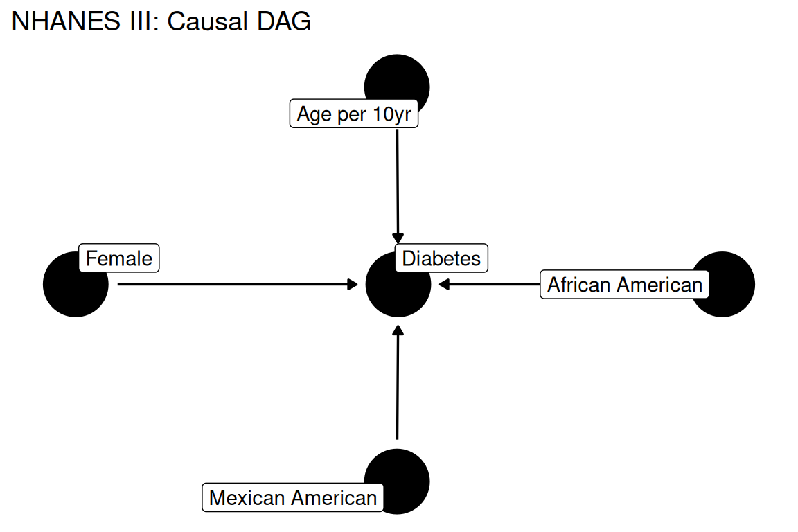
data(nhanes3, package = "rmb")
dat <- nhanes3
dim(dat)
#> [1] 18162     9
summary(haven::zap_labels(dat[c("diabetes", "female", "aframer", "mexamer", "age10")]))
#>     diabetes           female          aframer         mexamer
#>  Min.   :0.00000   Min.   :0.0000   Min.   :0.000   Min.   :0.0000
#>  1st Qu.:0.00000   1st Qu.:0.0000   1st Qu.:0.000   1st Qu.:0.0000
#>  Median :0.00000   Median :1.0000   Median :0.000   Median :0.0000
#>  Mean   :0.07387   Mean   :0.5327   Mean   :0.281   Mean   :0.2703
#>  3rd Qu.:0.00000   3rd Qu.:1.0000   3rd Qu.:1.000   3rd Qu.:1.0000
#>  Max.   :1.00000   Max.   :1.0000   Max.   :1.000   Max.   :1.0000
#>  NAs    :22
#>      age10
#>  Min.   :1.700
#>  1st Qu.:2.900
#>  Median :4.300
#>  Mean   :4.687
#>  3rd Qu.:6.400
#>  Max.   :9.000
#> A survey design object is constructed using PSUs, strata, and sampling weights, then survey-weighted logistic regression is fitted for diabetes on age (per 10 years), sex, African American ethnicity, and Mexican American ethnicity (RMB2e Ch. 12).
nhanes_design <- survey::svydesign(
  id = ~sdppsu6,
  strata = ~sdpstra6,
  weights = ~wtpfqx6,
  data = dat,
  nest = TRUE
)
formula_main <- diabetes ~ female + aframer + mexamer + age10
formula_main
#> diabetes ~ female + aframer + mexamer + age10survey::svymean(~diabetes, nhanes_design)
#> mean SE
#> diabetes NA NaN
survey::svyby(~diabetes, ~aframer, nhanes_design, survey::svymean)
#> aframer diabetes se
#> 0 0 NA NaN
#> 1 1 NA NaN
survey::svyby(~diabetes, ~mexamer, nhanes_design, survey::svymean)
#> mexamer diabetes se
#> 0 0 NA NaN
#> 1 1 NA NaNdm_by_age <- survey::svyby(~diabetes, ~age10, nhanes_design, survey::svymean)
ggplot2::ggplot(dm_by_age, ggplot2::aes(x = age10, y = diabetes)) +
ggplot2::geom_line(color = "#1b9e77", linewidth = 1) +
ggplot2::geom_point(color = "#1b9e77", size = 3) +
ggplot2::labs(
title = "NHANES III: Diabetes prevalence by age (survey-weighted)",
x = "Age group (per 10yr)",
y = "Weighted diabetes prevalence"
) +
ggplot2::theme_minimal()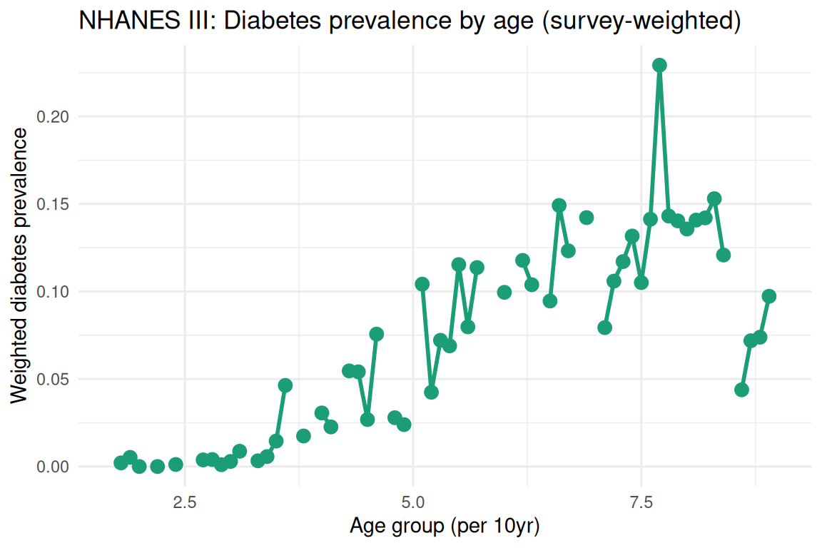
fit <- survey::svyglm(formula_main, design = nhanes_design, family = stats::binomial())
summary(fit)
#>
#> Call:
#> svyglm(formula = formula_main, design = nhanes_design, family = stats::binomial())
#>
#> Survey design:
#> survey::svydesign(id = ~sdppsu6, strata = ~sdpstra6, weights = ~wtpfqx6,
#>     data = dat, nest = TRUE)
#>
#> Coefficients:
#>             Estimate Std. Error t value Pr(>|t|)
#> (Intercept) -5.79408    0.19487 -29.733  < 2e-16 ***
#> female      -0.01954    0.09392  -0.208    0.836
#> aframer      0.59845    0.09508   6.294 1.14e-07 ***
#> mexamer      0.64715    0.09797   6.606 3.93e-08 ***
#> age10        0.53286    0.02774  19.211  < 2e-16 ***
#> ---
#> Signif. codes:  0 '***' 0.001 '**' 0.01 '*' 0.05 '.' 0.1 ' ' 1
#>
#> (Dispersion parameter for binomial family taken to be 0.8635979)
#>
#> Number of Fisher Scoring iterations: 6fit_age_only <- survey::svyglm(diabetes ~ age10, design = nhanes_design, family = stats::binomial())
stats::anova(fit_age_only, fit, test = "Chisq")
#> Working (Rao-Scott) LRT for female aframer mexamer
#> in svyglm(formula = formula_main, design = nhanes_design, family = stats::binomial())
#> Working 2logLR = 43.9424 p= 2.2564e-06
#> (scale factors: 1.9 0.87 0.24 )or <- exp(stats::coef(fit))
ci <- exp(stats::confint(fit))
data.frame(
term = names(or),
odds_ratio = unname(or),
conf_low = ci[, 1],
conf_high = ci[, 2],
p_value = summary(fit)$coefficients[, "Pr(>|t|)"]
)
#> term odds_ratio conf_low conf_high p_value
#> (Intercept) (Intercept) 0.003045541 0.002056872 0.004509432 3.160774e-31
#> female female 0.980651263 0.811642396 1.184852964 8.361362e-01
#> aframer aframer 1.819299812 1.502228919 2.203293896 1.141043e-07
#> mexamer mexamer 1.910096525 1.568047072 2.326759700 3.926636e-08
#> age10 age10 1.703792188 1.611221551 1.801681351 2.568224e-23Older age, African American ethnicity, and Mexican American ethnicity are all associated with higher diabetes prevalence in the US population after mutual adjustment, consistent with well-documented patterns of diabetes disparities (RMB2e Ch. 12). Using survey weights is essential: the complex NHANES III sampling design over-represents certain demographic groups, and unweighted estimates would misrepresent national prevalence. This analysis illustrates the survey-weighted GLM approach that is required whenever data come from complex probability samples with unequal selection probabilities.