Code
data(rmb_datasets, package = "rmb")
rmb_datasets$study_design[rmb_datasets$object == "hers_long_base_visit1_only_saved"]
#> [1] "Baseline/Visit 1 subset from the longitudinal HERS data structure."
This article analyzes glucose levels at Year-1 follow-up in HERS participants, examining how HRT assignment, exercise, and BMI relate to glycemic outcomes (RMB2e Chapter 11).
The Heart and Estrogen/Progestin Replacement Study (HERS) enrolled postmenopausal women with established coronary heart disease and randomized them to hormone therapy (HRT) or placebo. Beyond its primary cardiovascular endpoints, HERS collected repeated metabolic measurements including fasting glucose, enabling analysis of longitudinal glycemic trajectories. Missing data patterns in metabolic outcomes are a key methodological concern in longitudinal studies (RMB2e Chapter 11).
data(rmb_datasets, package = "rmb")
rmb_datasets$study_design[rmb_datasets$object == "hers_long_base_visit1_only_saved"]
#> [1] "Baseline/Visit 1 subset from the longitudinal HERS data structure."This dataset contains baseline and Visit 1 data from the HERS longitudinal structure. We ask: among women without diabetes at baseline, is HRT assignment associated with Year-1 fasting glucose after adjusting for exercise and BMI?
set.seed(42)
dag <- ggdag::dagify(
  gluc ~ hrt + bmi + exercise + age,
  bmi ~ age,
  labels = c(
    gluc = "Year-1 glucose",
    hrt = "HRT assignment",
    bmi = "BMI",
    exercise = "Exercise >=3x/wk",
    age = "Age"
  ),
  exposure = "hrt",
  outcome = "gluc"
)
ggdag::ggdag(dag, use_labels = "label", text = FALSE) +
  ggdag::theme_dag_blank() +
  ggplot2::labs(title = "HERS baseline: Causal DAG")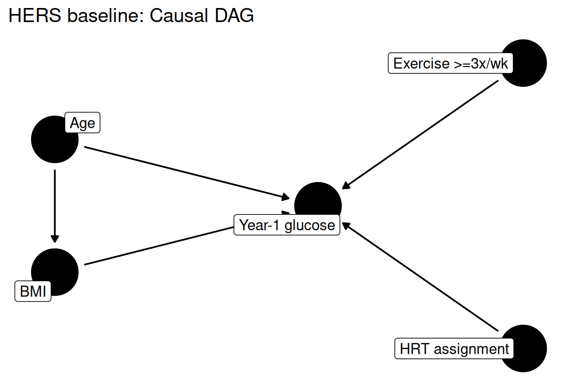
data(hers_long_base_visit1_only_saved, package = "rmb")
dat <- haven::zap_labels(hers_long_base_visit1_only_saved)
dim(dat)
#> [1] 5526   22
ana <- subset(dat, nvisit == 1 & diabetes == 0)
dim(ana)
#> [1] 1942   22
summary(ana[c("glucose", "group", "bmi", "exer3", "age")])
#>     glucose           group             bmi            exer3
#>  Min.   : 62.00   Min.   :0.0000   Min.   :14.73   Min.   :0.0000
#>  1st Qu.: 89.00   1st Qu.:0.0000   1st Qu.:23.85   1st Qu.:0.0000
#>  Median : 96.00   Median :0.0000   Median :26.77   Median :0.0000
#>  Mean   : 96.74   Mean   :0.4943   Mean   :27.47   Mean   :0.3845
#>  3rd Qu.:103.00   3rd Qu.:1.0000   3rd Qu.:30.26   3rd Qu.:1.0000
#>  Max.   :125.00   Max.   :1.0000   Max.   :52.78   Max.   :1.0000
#>  NAs    :11                        NAs    :14      NAs    :7
#>       age
#>  Min.   :44.00
#>  1st Qu.:62.00
#>  Median :68.00
#>  Mean   :66.94
#>  3rd Qu.:72.00
#>  Max.   :79.00
#> We fit a linear regression model for Year-1 fasting glucose with HRT assignment (group) as the primary predictor, adjusting for BMI, exercise frequency, age, and smoking status among women attending Visit 1 without diabetes.
formula_gluc <- glucose ~ group + bmi + exer3 + age + csmker
formula_gluc
#> glucose ~ group + bmi + exer3 + age + csmkerwith(ana, tapply(glucose, group, summary))
#> $`0`
#> Min. 1st Qu. Median Mean 3rd Qu. Max. NAs
#> 62.00 91.00 97.00 98.01 104.00 125.00 3
#>
#> $`1`
#> Min. 1st Qu. Median Mean 3rd Qu. Max. NAs
#> 68.00 88.00 94.00 95.44 101.25 125.00 8
with(ana, tapply(glucose, exer3, mean, na.rm = TRUE))
#> 0 1
#> 97.26796 95.93252ana$group_label <- factor(ana$group, levels = c(0, 1), labels = c("Placebo", "HRT"))
ggplot2::ggplot(ana, ggplot2::aes(x = group_label, y = glucose, fill = group_label)) +
ggplot2::geom_boxplot() +
ggplot2::scale_fill_manual(values = c("grey85", "#d95f02")) +
ggplot2::labs(
title = "HERS: Year-1 glucose by HRT assignment",
x = "Treatment assignment",
y = "Year-1 fasting glucose (mg/dL)"
) +
ggplot2::theme_minimal() +
ggplot2::theme(legend.position = "none")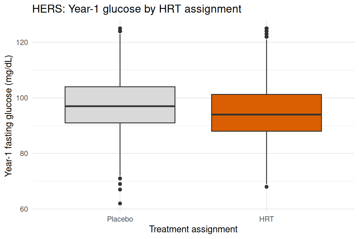
fit_gluc <- stats::lm(formula_gluc, data = ana)
summary(fit_gluc)
#>
#> Call:
#> stats::lm(formula = formula_gluc, data = ana)
#>
#> Residuals:
#>     Min      1Q  Median      3Q     Max
#> -32.714  -6.846  -0.915   6.011  31.057
#>
#> Coefficients:
#>             Estimate Std. Error t value Pr(>|t|)
#> (Intercept) 77.29712    2.95896  26.123  < 2e-16 ***
#> group       -2.29360    0.45644  -5.025 5.51e-07 ***
#> bmi          0.55186    0.04562  12.097  < 2e-16 ***
#> exer3       -0.58024    0.47661  -1.217   0.2236
#> age          0.08253    0.03549   2.326   0.0201 *
#> csmker       0.71728    0.64456   1.113   0.2659
#> ---
#> Signif. codes:  0 '***' 0.001 '**' 0.01 '*' 0.05 '.' 0.1 ' ' 1
#>
#> Residual standard error: 9.987 on 1912 degrees of freedom
#>   (24 observations deleted due to missingness)
#> Multiple R-squared:  0.0879, Adjusted R-squared:  0.08552
#> F-statistic: 36.85 on 5 and 1912 DF, p-value: < 2.2e-16fit_data <- data.frame(
fitted = stats::fitted(fit_gluc),
residuals = stats::residuals(fit_gluc),
std_residuals = stats::rstandard(fit_gluc)
)
ggplot2::ggplot(fit_data, ggplot2::aes(x = fitted, y = residuals)) +
ggplot2::geom_point(alpha = 0.25, size = 0.5) +
ggplot2::geom_hline(yintercept = 0, linetype = "dashed", color = "red") +
ggplot2::geom_smooth(se = FALSE, color = "blue") +
ggplot2::labs(
title = "Residuals vs Fitted",
x = "Fitted values",
y = "Residuals"
) +
ggplot2::theme_minimal()
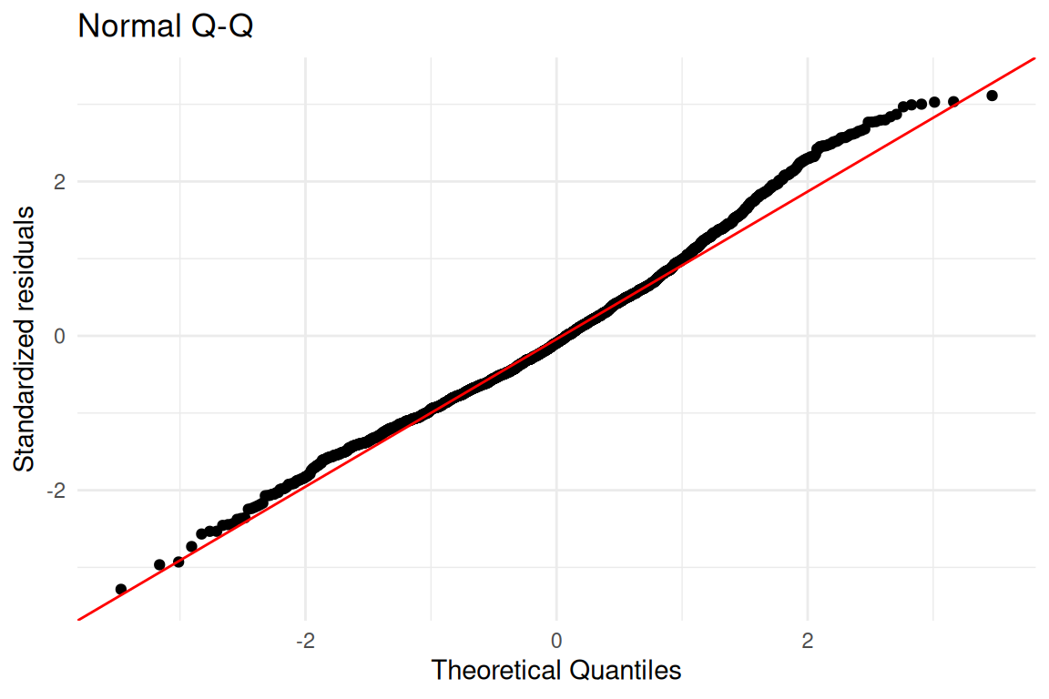
ggplot2::ggplot(fit_data, ggplot2::aes(sample = std_residuals)) +
ggplot2::stat_qq() +
ggplot2::stat_qq_line(color = "red") +
ggplot2::labs(
title = "Normal Q-Q",
x = "Theoretical Quantiles",
y = "Standardized residuals"
) +
ggplot2::theme_minimal()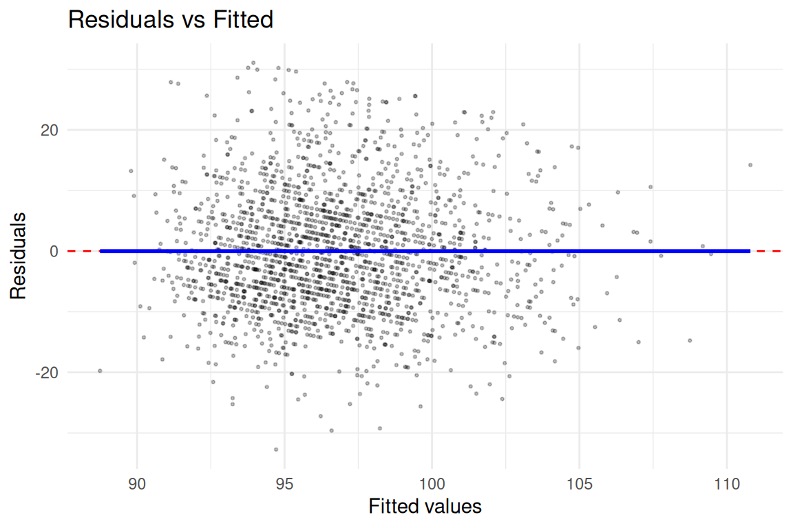
ci <- stats::confint(fit_gluc)
coef_tab <- data.frame(
  term = names(stats::coef(fit_gluc)),
  estimate = stats::coef(fit_gluc),
  conf_low = ci[, 1],
  conf_high = ci[, 2],
  p_value = summary(fit_gluc)$coefficients[, "Pr(>|t|)"]
)
coef_tab
#>                    term    estimate    conf_low  conf_high       p_value
#> (Intercept) (Intercept) 77.29711774 71.49398627 83.1002492 6.782014e-129
#> group             group -2.29360213 -3.18878237 -1.3984219  5.505243e-07
#> bmi                 bmi  0.55185745  0.46238486  0.6413300  1.641742e-32
#> exer3             exer3 -0.58023656 -1.51497570  0.3545026  2.235975e-01
#> age                 age  0.08252925  0.01292922  0.1521293  2.014789e-02
#> csmker csmker 0.71728209 -0.54682682 1.9813910 2.659216e-01In this HERS baseline/Visit-1 longitudinal analysis, HRT assignment does not appear to substantially change fasting glucose in women without diabetes after adjustment for BMI, exercise, and age. The analysis illustrates the longitudinal data structure used in RMB2e Chapter 11 for missing-data examples, where patterns of missingness in glucose are related to baseline characteristics. Regular exercise is associated with lower glucose levels, consistent with its known metabolic effects.