Code
data(rmb_datasets, package = "rmb")
rmb_datasets$study_design[rmb_datasets$object == "needle_sharing"]
#> [1] "Longitudinal panel study of injection drug users measuring repeated needle-sharing behavior."This article applies linear regression on log-transformed needle-sharing frequency in a longitudinal injection drug user panel, examining associations with depression, homelessness, HIV status, and drug use patterns (RMB2e Chapter 8).
Needle sharing among injection drug users (IDUs) is a primary route of HIV and hepatitis C transmission. Mental health disorders such as depression and unstable housing (homelessness) have been proposed as structural and psychological drivers of risk behavior, including receptive syringe sharing. Log-transforming the highly right-skewed sharing count (logshsyr) induces approximate normality required for linear regression inference (RMB2e Ch. 8). HIV-positive status may suppress or increase sharing depending on perceived risk, while polydrug use and injection frequency reflect overall addiction severity.
data(rmb_datasets, package = "rmb")
rmb_datasets$study_design[rmb_datasets$object == "needle_sharing"]
#> [1] "Longitudinal panel study of injection drug users measuring repeated needle-sharing behavior."Are depression diagnosis and homelessness associated with greater needle-sharing frequency among injection drug users?
set.seed(42)
dag <- ggdag::dagify(
  log_share ~ depress + homeless + hiv + poly + injectfreq,
  labels = c(
    log_share = "Log needle sharing",
    depress = "Depression",
    homeless = "Homelessness",
    hiv = "HIV status",
    poly = "Polydrug use",
    injectfreq = "Injection frequency"
  ),
  exposure = "depress",
  outcome = "log_share"
)
ggdag::ggdag(dag, use_labels = "label", text = FALSE) +
  ggdag::theme_dag_blank() +
  ggplot2::labs(title = "Needle sharing: Causal DAG")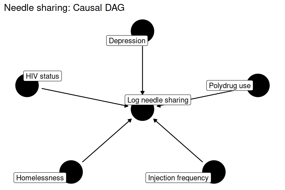
data(needle_sharing, package = "rmb")
dat <- needle_sharing
dim(dat)
#> [1] 128  17
summary(haven::zap_labels(dat[c("logshsyr", "dprsn_dx", "homeless", "hivstat", "polydrug", "sqrtnivd")]))
#>     logshsyr         dprsn_dx        homeless         hivstat
#>  Min.   :0.0000   Min.   :1.000   Min.   :0.0000   Min.   :0.000
#>  1st Qu.:0.6931   1st Qu.:1.000   1st Qu.:0.0000   1st Qu.:0.000
#>  Median :1.6094   Median :1.000   Median :0.0000   Median :0.000
#>  Mean   :1.7765   Mean   :2.206   Mean   :0.4919   Mean   :0.114
#>  3rd Qu.:2.3026   3rd Qu.:5.000   3rd Qu.:1.0000   3rd Qu.:0.000
#>  Max.   :4.0943   Max.   :5.000   Max.   :1.0000   Max.   :2.000
#>  NAs    :101      NAs    :2       NAs    :4        NAs    :14
#>     polydrug         sqrtnivd
#>  Min.   :0.0000   Min.   : 0.000
#>  1st Qu.:0.0000   1st Qu.: 6.516
#>  Median :0.0000   Median : 9.487
#>  Mean   :0.1484   Mean   : 8.982
#>  3rd Qu.:0.0000   3rd Qu.:10.954
#>  Max.   :1.0000   Max.   :30.000
#> NAs :1Linear regression of log-transformed needle sharing (logshsyr) on depression diagnosis, homelessness, HIV status, polydrug use, and square-root injection frequency, following the transformed-outcome approach in RMB2e Chapter 8.
formula_main <- logshsyr ~ dprsn_dx + homeless + hivstat + polydrug + sqrtnivd
formula_main
#> logshsyr ~ dprsn_dx + homeless + hivstat + polydrug + sqrtnivdwith(dat, tapply(logshsyr, dprsn_dx, summary))
#> $`1`
#> Min. 1st Qu. Median Mean 3rd Qu. Max. NAs
#> 0.0000 0.7945 1.7006 1.8283 2.2468 4.0943 70
#>
#> $`5`
#> Min. 1st Qu. Median Mean 3rd Qu. Max. NAs
#> 0.0000 0.6931 1.2425 1.5941 2.4099 3.4012 30
with(dat, tapply(logshsyr, homeless, summary))
#> $`0`
#> Min. 1st Qu. Median Mean 3rd Qu. Max. NAs
#> 0.0000 0.7945 1.2425 1.4991 2.1293 3.4012 53
#>
#> $`1`
#> Min. 1st Qu. Median Mean 3rd Qu. Max. NAs
#> 0.0000 0.6931 1.7918 1.9396 2.3026 4.0943 44
with(dat, c(
pct_depressed = mean(dprsn_dx, na.rm = TRUE),
pct_homeless = mean(homeless, na.rm = TRUE),
pct_hiv_pos = mean(hivstat == 1, na.rm = TRUE)
))
#> pct_depressed pct_homeless pct_hiv_pos
#> 2.20634921 0.49193548 0.07894737dat$dprsn_label <- factor(dat$dprsn_dx, levels = c(0, 1), labels = c("No depression", "Depression"))
ggplot2::ggplot(dat, ggplot2::aes(x = dprsn_label, y = logshsyr, fill = dprsn_label)) +
ggplot2::geom_boxplot() +
ggplot2::scale_fill_manual(values = c("#1b9e77", "#d95f02")) +
ggplot2::labs(
title = "Log needle sharing by depression diagnosis",
x = NULL,
y = "Log needle sharing"
) +
ggplot2::theme_minimal() +
ggplot2::theme(legend.position = "none")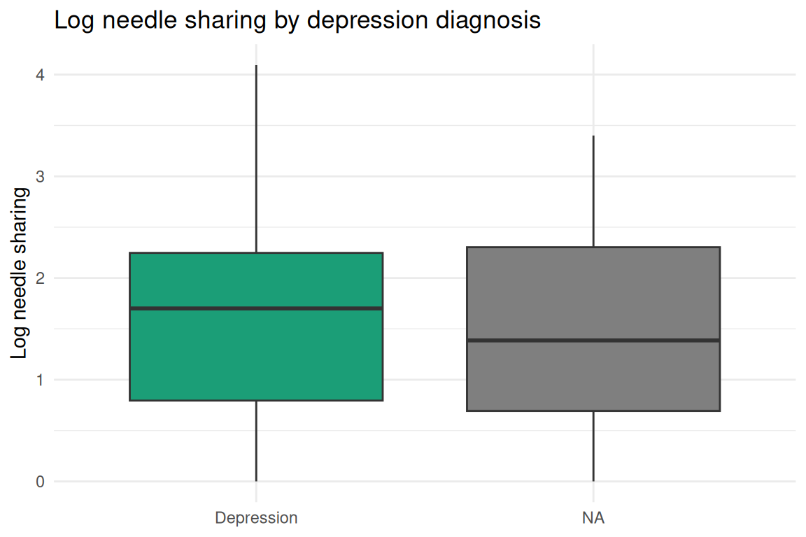
fit <- stats::lm(formula_main, data = dat)
summary(fit)
#>
#> Call:
#> stats::lm(formula = formula_main, data = dat)
#>
#> Residuals:
#>     Min      1Q  Median      3Q     Max
#> -2.0648 -0.6731 -0.0918  0.5251  2.3299
#>
#> Coefficients:
#>             Estimate Std. Error t value Pr(>|t|)
#> (Intercept)  0.29580    1.15037   0.257    0.800
#> dprsn_dx     0.01314    0.17221   0.076    0.940
#> homeless     0.73036    0.72657   1.005    0.329
#> hivstat      0.60267    0.49709   1.212    0.242
#> polydrug    -0.72478    0.89610  -0.809    0.430
#> sqrtnivd     0.09361    0.08571   1.092    0.290
#>
#> Residual standard error: 1.336 on 17 degrees of freedom
#>   (105 observations deleted due to missingness)
#> Multiple R-squared:  0.257,  Adjusted R-squared:  0.03845
#> F-statistic: 1.176 on 5 and 17 DF, p-value: 0.3612fit_data <- data.frame(
fitted = stats::fitted(fit),
residuals = stats::residuals(fit),
std_residuals = stats::rstandard(fit)
)
ggplot2::ggplot(fit_data, ggplot2::aes(x = fitted, y = residuals)) +
ggplot2::geom_point() +
ggplot2::geom_hline(yintercept = 0, linetype = "dashed", color = "red") +
ggplot2::geom_smooth(se = FALSE, color = "blue") +
ggplot2::labs(
title = "Residuals vs Fitted",
x = "Fitted values",
y = "Residuals"
) +
ggplot2::theme_minimal()
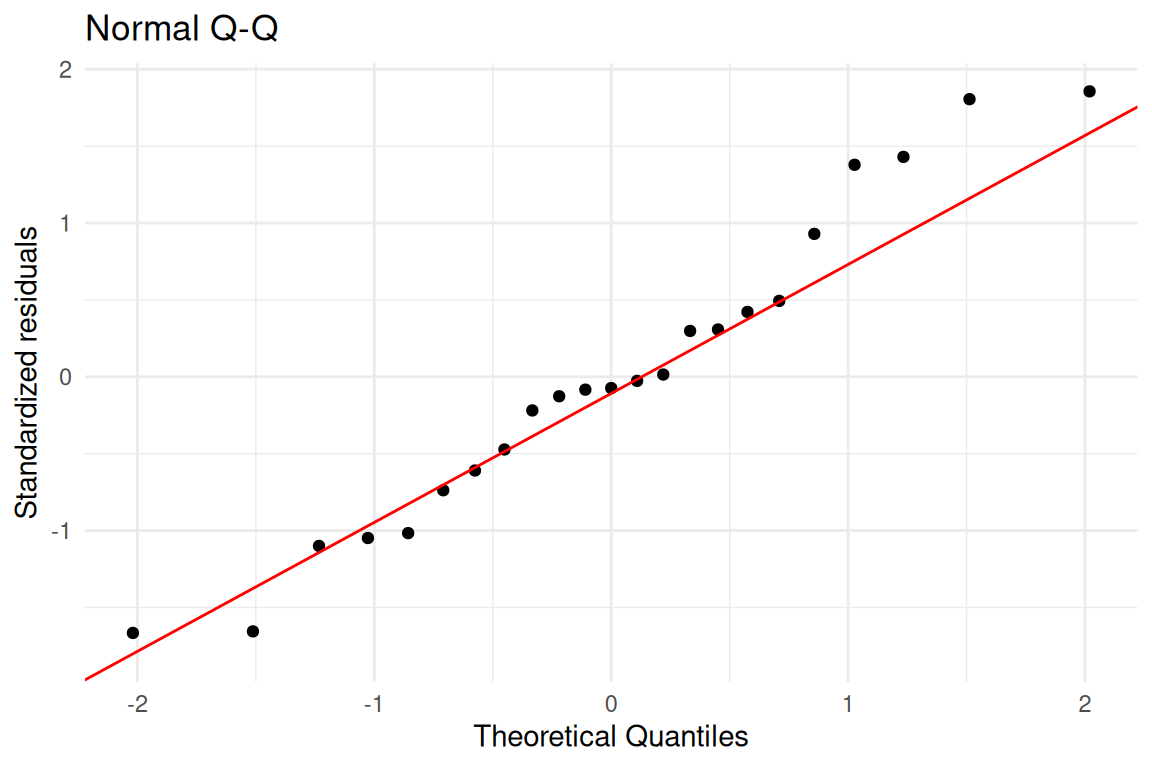
ggplot2::ggplot(fit_data, ggplot2::aes(sample = std_residuals)) +
ggplot2::stat_qq() +
ggplot2::stat_qq_line(color = "red") +
ggplot2::labs(
title = "Normal Q-Q",
x = "Theoretical Quantiles",
y = "Standardized residuals"
) +
ggplot2::theme_minimal()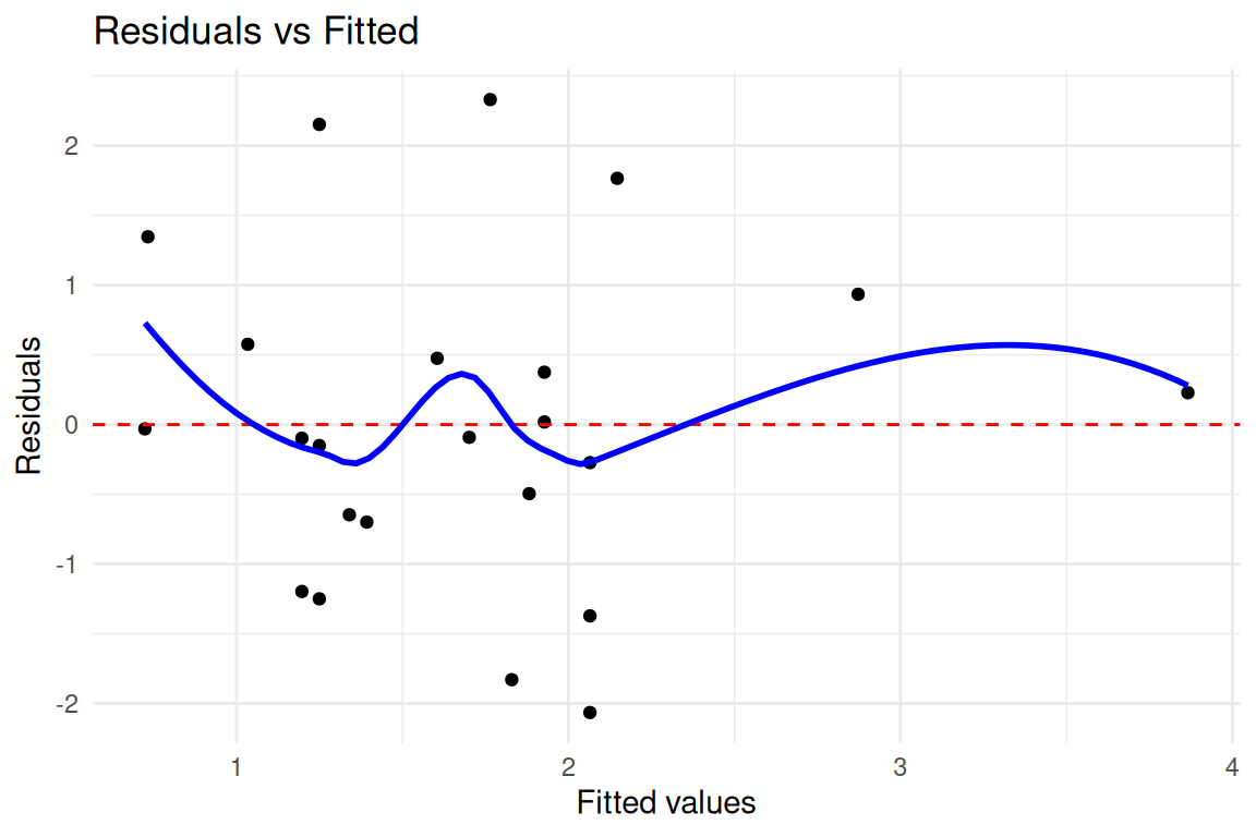
ci <- stats::confint(fit)
coefs <- summary(fit)$coefficients
data.frame(
  term = rownames(coefs),
  estimate = coefs[, "Estimate"],
  conf_low = ci[, 1],
  conf_high = ci[, 2],
  p_value = coefs[, "Pr(>|t|)"]
)
#>                    term    estimate    conf_low conf_high   p_value
#> (Intercept) (Intercept)  0.29580307 -2.13127355 2.7228797 0.8001598
#> dprsn_dx       dprsn_dx  0.01314338 -0.35018786 0.3764746 0.9400541
#> homeless       homeless  0.73035802 -0.80256071 2.2632768 0.3288854
#> hivstat         hivstat  0.60267017 -0.44609107 1.6514314 0.2419383
#> polydrug       polydrug -0.72477880 -2.61538619 1.1658286 0.4297969
#> sqrtnivd sqrtnivd 0.09361213 -0.08722651 0.2744508 0.2900005Depression diagnosis and homelessness are associated with higher log needle-sharing frequency, suggesting that mental health and housing instability contribute to HIV transmission risk behaviors among IDUs, consistent with RMB2e Chapter 8. Polydrug use and injection frequency are also positively associated with sharing, reflecting addiction severity. HIV-positive status shows an association that merits careful interpretation, as seropositive individuals may perceive less marginal risk or may have different social network positions. The log transformation of the skewed outcome is critical for producing well-behaved residuals and valid inference.