Code
data(rmb_datasets, package = "rmb")
rmb_datasets$study_design[rmb_datasets$object == "fitdata"]
#> [1] "Longitudinal FIT subset focused on bone mineral density outcomes."This article uses the longitudinal FIT dataset to assess whether alendronate treatment is associated with greater end-of-study femoral neck BMD, adjusting for baseline BMD and key risk factors (RMB2e Chapter 9).
The Fracture Intervention Trial (FIT) collected femoral neck BMD at both baseline and end-of-study, enabling assessment of treatment-related BMD change alongside fracture endpoints. Bisphosphonates such as alendronate inhibit osteoclast-mediated bone resorption, thereby increasing BMD; however, the magnitude of BMD gain depends on baseline BMD, fracture history, and patient characteristics. Linear regression on end-of-study BMD with baseline BMD as a covariate (analysis of covariance) is the appropriate approach for estimating treatment effects on a continuous outcome in a randomized trial (RMB2e Ch. 9 / Black 1996).
data(rmb_datasets, package = "rmb")
rmb_datasets$study_design[rmb_datasets$object == "fitdata"]
#> [1] "Longitudinal FIT subset focused on bone mineral density outcomes."Is alendronate treatment associated with greater end-of-study femoral neck BMD from baseline, after adjustment for baseline BMD, age, BMI, and prior vertebral fracture?
set.seed(42)
dag <- ggdag::dagify(
  cobmd ~ tx + blbmd + age + bmi + blvfx,
  labels = c(
    cobmd = "End BMD",
    tx = "Alendronate",
    blbmd = "Baseline BMD",
    age = "Age",
    bmi = "BMI",
    blvfx = "Prior fx"
  ),
  exposure = "tx",
  outcome = "cobmd"
)
ggdag::ggdag(dag, use_labels = "label", text = FALSE) +
  ggdag::theme_dag_blank() +
  ggplot2::labs(title = "FIT data: Causal DAG")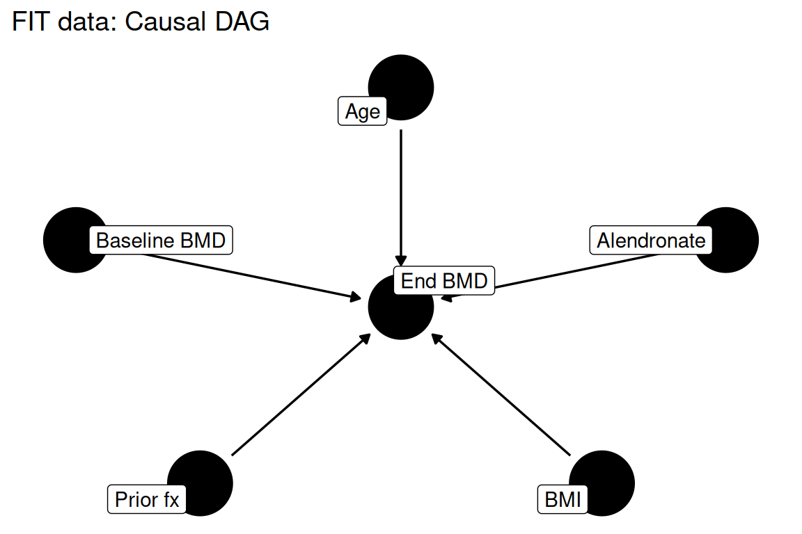
data(fitdata, package = "rmb")
dat <- fitdata
dim(dat)
#> [1] 5813   10
summary(haven::zap_labels(dat[c("tx", "blbmd", "cobmd", "age", "bmi", "blvfx")]))
#>        tx             blbmd            cobmd             age
#>  Min.   :0.0000   Min.   :0.3460   Min.   :0.3410   Min.   :55.05
#>  1st Qu.:0.0000   1st Qu.:0.5420   1st Qu.:0.5450   1st Qu.:64.04
#>  Median :1.0000   Median :0.5910   Median :0.5990   Median :68.44
#>  Mean   :0.5008   Mean   :0.5845   Mean   :0.5935   Mean   :68.35
#>  3rd Qu.:1.0000   3rd Qu.:0.6350   3rd Qu.:0.6450   3rd Qu.:72.83
#>  Max.   :1.0000   Max.   :0.7830   Max.   :0.9020   Max.   :81.87
#>                   NAs    :1        NAs    :401
#>       bmi            blvfx
#>  Min.   :15.66   Min.   :0.0000
#>  1st Qu.:22.36   1st Qu.:0.0000
#>  Median :24.60   Median :0.0000
#>  Mean   :25.14   Mean   :0.3112
#>  3rd Qu.:27.33   3rd Qu.:1.0000
#>  Max.   :47.77   Max.   :1.0000
#> A linear model regresses end-of-study femoral neck BMD (cobmd) on treatment assignment (tx), baseline BMD (blbmd), age, BMI, and prior vertebral fracture history (blvfx), following the analysis of covariance approach recommended in RMB2e Chapter 9.
formula_main <- cobmd ~ tx + blbmd + age + bmi + blvfx
formula_main
#> cobmd ~ tx + blbmd + age + bmi + blvfxwith(dat, tapply(cobmd, tx, summary))
#> $`0`
#> Min. 1st Qu. Median Mean 3rd Qu. Max. NAs
#> 0.3410 0.5370 0.5840 0.5803 0.6300 0.8220 188
#>
#> $`1`
#> Min. 1st Qu. Median Mean 3rd Qu. Max. NAs
#> 0.3490 0.5590 0.6120 0.6067 0.6590 0.9020 213
with(dat, tapply(blbmd, tx, summary))
#> $`0`
#> Min. 1st Qu. Median Mean 3rd Qu. Max. NAs
#> 0.3460 0.5410 0.5910 0.5846 0.6360 0.7470 1
#>
#> $`1`
#> Min. 1st Qu. Median Mean 3rd Qu. Max.
#> 0.3540 0.5430 0.5910 0.5845 0.6340 0.7830
with(dat, cor(cbind(cobmd, blbmd, age, bmi), use = "complete.obs"))
#> cobmd blbmd age bmi
#> cobmd 1.0000000 0.8747806 -0.21647925 0.29019704
#> blbmd 0.8747806 1.0000000 -0.22241441 0.27429061
#> age -0.2164792 -0.2224144 1.00000000 0.01479795
#> bmi 0.2901970 0.2742906 0.01479795 1.00000000dat$tx_label <- factor(dat$tx, levels = c(0, 1), labels = c("Placebo", "Alendronate"))
ggplot2::ggplot(dat, ggplot2::aes(x = blbmd, y = cobmd, color = tx_label)) +
ggplot2::geom_point(alpha = 0.6, size = 0.8) +
ggplot2::scale_color_manual(values = c("#1b9e77", "#d95f02")) +
ggplot2::labs(
title = "FIT: End BMD vs baseline BMD by treatment",
x = "Baseline femoral neck BMD (g/cm²)",
y = "End-of-study femoral neck BMD (g/cm²)",
color = NULL
) +
ggplot2::theme_minimal() +
ggplot2::theme(legend.position = c(0.15, 0.9))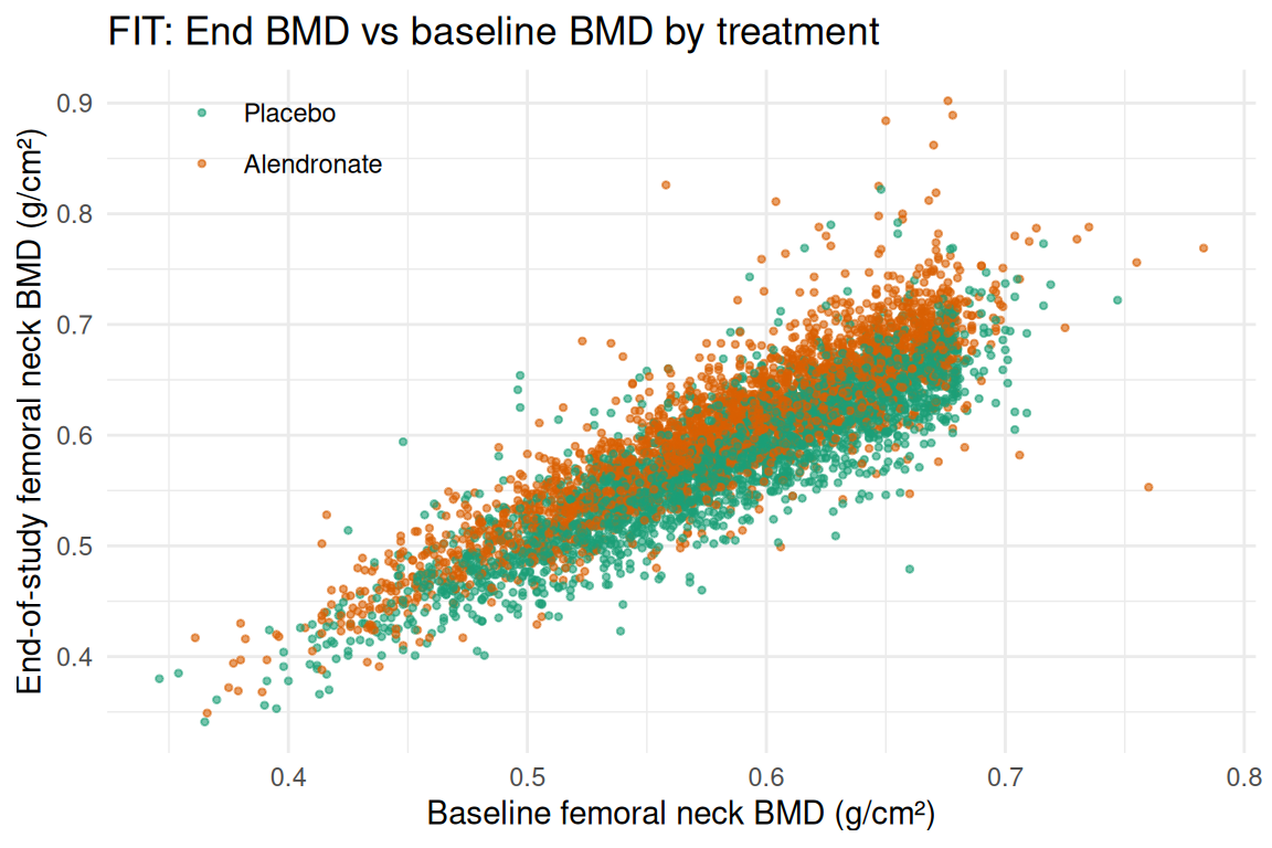
fit_model <- stats::lm(formula_main, data = dat)
summary(fit_model)
#>
#> Call:
#> stats::lm(formula = formula_main, data = dat)
#>
#> Residuals:
#>       Min        1Q    Median        3Q       Max
#> -0.223866 -0.018384 -0.000967  0.017608  0.248120
#>
#> Coefficients:
#>               Estimate Std. Error t value Pr(>|t|)
#> (Intercept)  1.276e-02  7.244e-03   1.761 0.078310 .
#> tx           2.666e-02  8.612e-04  30.959  < 2e-16 ***
#> blbmd        9.575e-01  7.367e-03 129.973  < 2e-16 ***
#> age         -2.754e-04  7.488e-05  -3.678 0.000237 ***
#> bmi          1.051e-03  1.130e-04   9.295  < 2e-16 ***
#> blvfx       -1.218e-03  9.768e-04  -1.246 0.212653
#> ---
#> Signif. codes:  0 '***' 0.001 '**' 0.01 '*' 0.05 '.' 0.1 ' ' 1
#>
#> Residual standard error: 0.03167 on 5405 degrees of freedom
#>   (402 observations deleted due to missingness)
#> Multiple R-squared:  0.8036, Adjusted R-squared:  0.8034
#> F-statistic: 4422 on 5 and 5405 DF, p-value: < 2.2e-16fit_data <- data.frame(
fitted = stats::fitted(fit_model),
residuals = stats::residuals(fit_model),
std_residuals = stats::rstandard(fit_model)
)
ggplot2::ggplot(fit_data, ggplot2::aes(x = fitted, y = residuals)) +
ggplot2::geom_point(alpha = 0.25, size = 0.5) +
ggplot2::geom_hline(yintercept = 0, linetype = "dashed", color = "red") +
ggplot2::geom_smooth(se = FALSE, color = "blue") +
ggplot2::labs(
title = "Residuals vs Fitted",
x = "Fitted values",
y = "Residuals"
) +
ggplot2::theme_minimal()
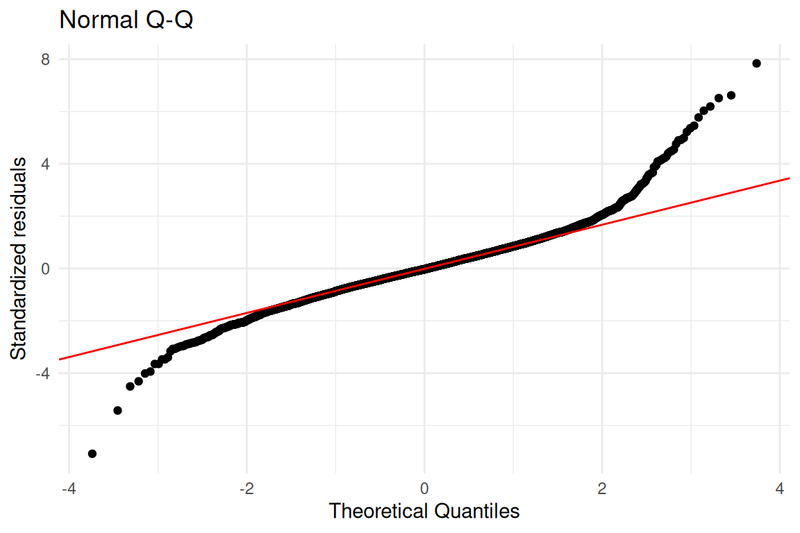
ggplot2::ggplot(fit_data, ggplot2::aes(sample = std_residuals)) +
ggplot2::stat_qq() +
ggplot2::stat_qq_line(color = "red") +
ggplot2::labs(
title = "Normal Q-Q",
x = "Theoretical Quantiles",
y = "Standardized residuals"
) +
ggplot2::theme_minimal()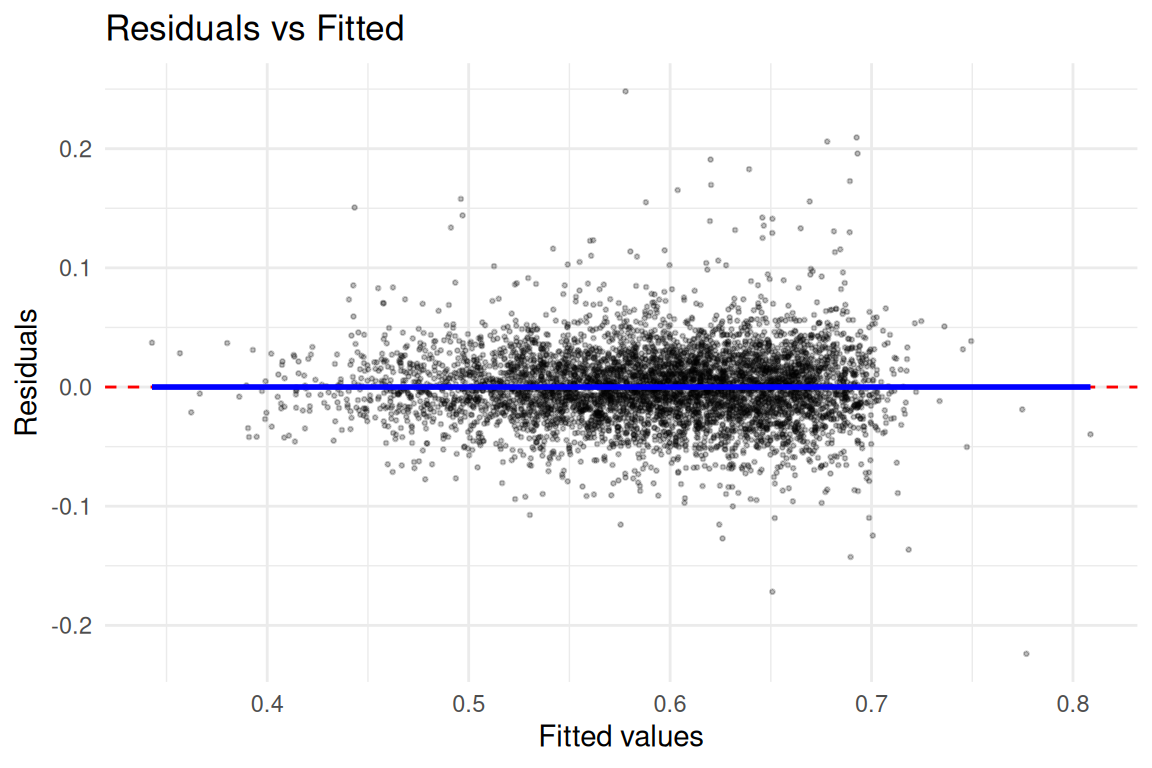
ci <- stats::confint(fit_model)
coefs <- summary(fit_model)$coefficients
data.frame(
  term = rownames(coefs),
  estimate = coefs[, "Estimate"],
  conf_low = ci[, 1],
  conf_high = ci[, 2],
  p_value = coefs[, "Pr(>|t|)"]
)
#>                    term     estimate      conf_low     conf_high       p_value
#> (Intercept) (Intercept)  0.012755895 -0.0014451101  0.0269568999  7.831015e-02
#> tx                   tx  0.026662103  0.0249737768  0.0283504295 7.051282e-194
#> blbmd             blbmd  0.957548434  0.9431056039  0.9719912647  0.000000e+00
#> age                 age -0.000275415 -0.0004222195 -0.0001286106  2.374956e-04
#> bmi                 bmi  0.001050524  0.0008289485  0.0012721005  2.096443e-20
#> blvfx blvfx -0.001217504 -0.0031323802 0.0006973712 2.126527e-01Alendronate treatment is positively associated with end-of-study femoral neck BMD after adjustment for baseline BMD and clinical characteristics, consistent with the mechanism of bisphosphonate action and the primary findings of Black et al. (1996). Baseline BMD is the dominant predictor of end-of-study BMD, as expected from the high autocorrelation of bone density measurements. This analysis of covariance design (with baseline BMD as covariate) is the recommended approach for estimating treatment effects on a continuous outcome in a randomized trial with heterogeneous baseline values (RMB2e Ch. 9).