Code
data(rmb_datasets, package = "rmb")
rmb_datasets$study_design[rmb_datasets$object == "sof2"]
#> [1] "Longitudinal repeated-measures subset of SOF focused on bone mineral density outcomes."This article models longitudinal total BMD trajectories in the SOF cohort using spline basis terms for visit time, testing whether late menopause modifies the rate of BMD decline (RMB2e Chapter 7).
Total bone mineral density in older women declines after menopause, but the trajectory need not be linear across follow-up years— the rate of loss may accelerate or decelerate over time. The SOF2 dataset extends the baseline SOF data with spline basis terms (visit_spl1, visit_spl2) encoding the nonlinear shape of BMD change over visits, and includes an indicator of late menopause (after age 52) as a potential modifier of longitudinal decline (RMB2e Ch. 7). A marginal model for repeated BMD captures the average population trajectory.
data(rmb_datasets, package = "rmb")
rmb_datasets$study_design[rmb_datasets$object == "sof2"]
#> [1] "Longitudinal repeated-measures subset of SOF focused on bone mineral density outcomes."How does total BMD change over follow-up visits, and is the rate of decline modified by late menopause?
set.seed(42)
dag <- ggdag::dagify(
  tbmd ~ bmdbase + bmi + time + menop,
  labels = c(
    tbmd = "Total BMD",
    bmdbase = "Baseline BMD",
    bmi = "BMI",
    time = "Visit/time",
    menop = "Late menopause"
  ),
  exposure = "menop",
  outcome = "tbmd"
)
ggdag::ggdag(dag, use_labels = "label", text = FALSE) +
  ggdag::theme_dag_blank() +
  ggplot2::labs(title = "SOF2: Causal DAG")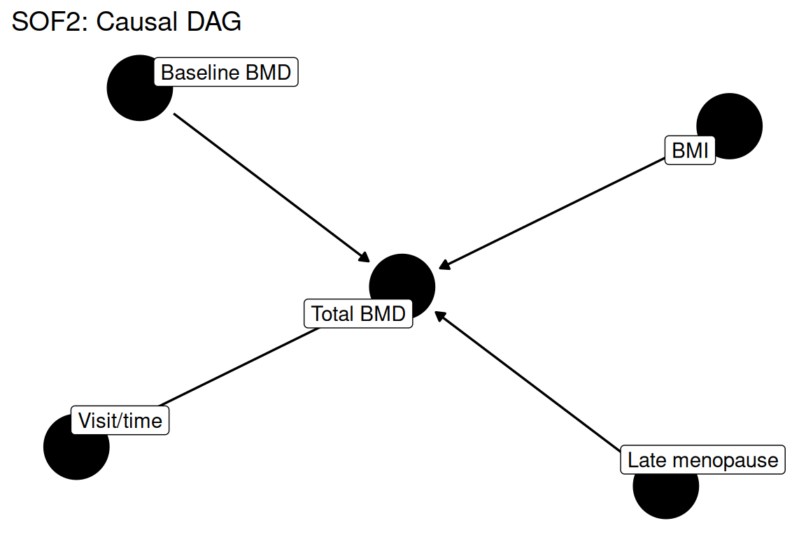
data(sof2, package = "rmb")
dat <- sof2
dim(dat)
#> [1] 42950    15
summary(haven::zap_labels(dat[c("totbmd", "base_totbmd", "bmi", "visit_spl1", "visit_spl2", "meno_ov_52")]))
#>      totbmd        base_totbmd          bmi          visit_spl1
#>  Min.   :0.1810   Min.   :0.3000   Min.   :13.00   Min.   :2
#>  1st Qu.:0.6459   1st Qu.:0.6592   1st Qu.:23.00   1st Qu.:4
#>  Median :0.7286   Median :0.7407   Median :26.00   Median :5
#>  Mean   :0.7352   Mean   :0.7470   Mean   :26.42   Mean   :5
#>  3rd Qu.:0.8170   3rd Qu.:0.8268   3rd Qu.:29.00   3rd Qu.:6
#>  Max.   :1.6553   Max.   :1.4030   Max.   :54.00   Max.   :8
#>  NAs    :15548    NAs    :1885     NAs    :16121
#>    visit_spl2       meno_ov_52
#>  Min.   :0.0000   Min.   :0.0000
#>  1st Qu.:0.2222   1st Qu.:0.0000
#>  Median :0.7500   Median :0.0000
#>  Mean   :1.4389   Mean   :0.1892
#>  3rd Qu.:1.7222   3rd Qu.:0.0000
#>  Max.   :4.5000   Max.   :1.0000
#> NAs :7930A marginal linear model regresses total BMD on baseline BMD, BMI, spline basis terms for visit, and late menopause indicator, estimating average BMD trajectories (RMB2e Ch. 7). Standard errors from this pooled OLS model do not account for within-subject correlation, but the model illustrates the approach before mixed-effects extensions.
formula_main <- totbmd ~ base_totbmd + bmi + visit_spl1 + visit_spl2 + meno_ov_52
formula_main
#> totbmd ~ base_totbmd + bmi + visit_spl1 + visit_spl2 + meno_ov_52visit_means <- with(dat, tapply(totbmd, visit, mean, na.rm = TRUE))
visit_df <- data.frame(
visit = as.integer(names(visit_means)),
mean_bmd = as.numeric(visit_means)
)
ggplot2::ggplot(visit_df, ggplot2::aes(x = visit, y = mean_bmd)) +
ggplot2::geom_line(color = "#1b9e77", linewidth = 1) +
ggplot2::geom_point(color = "#1b9e77", size = 3) +
ggplot2::labs(
title = "SOF2: Mean total BMD by visit",
x = "Visit number",
y = "Mean total BMD (g/cm²)"
) +
ggplot2::theme_minimal()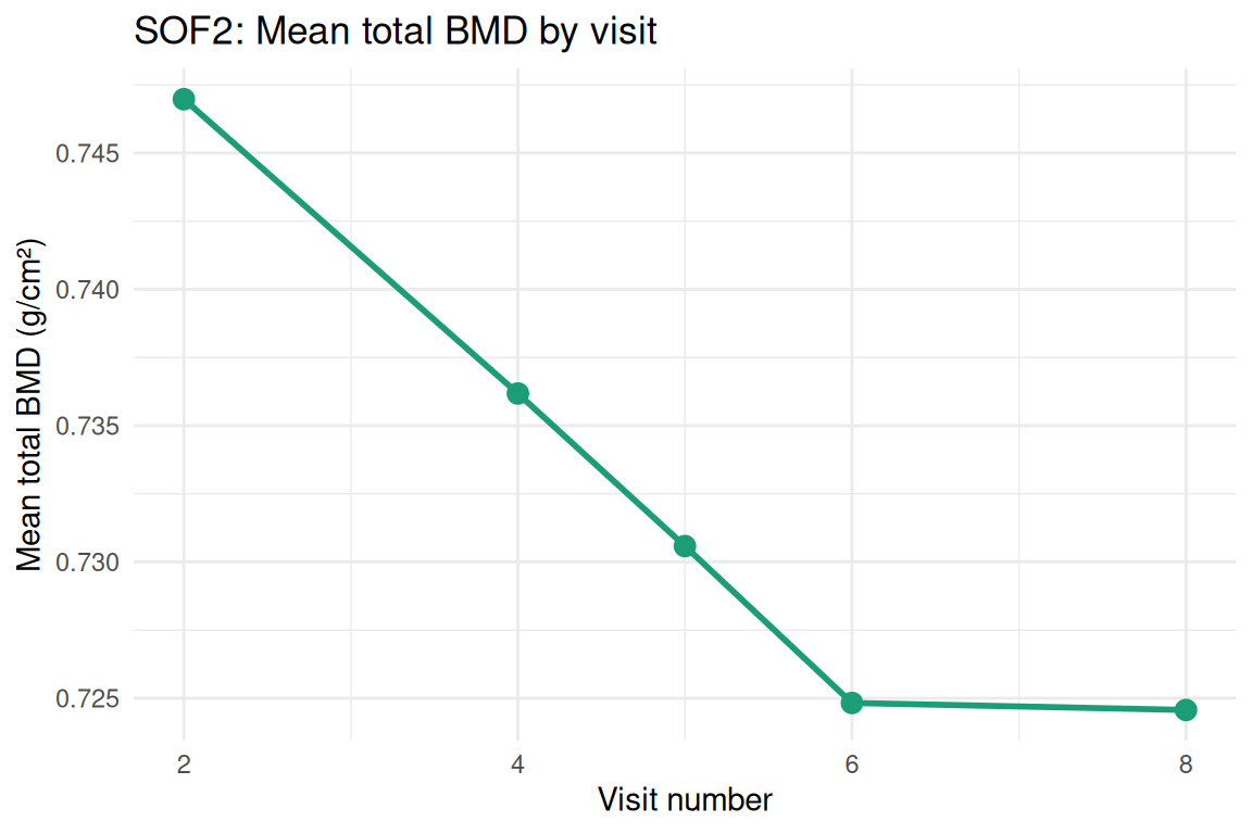
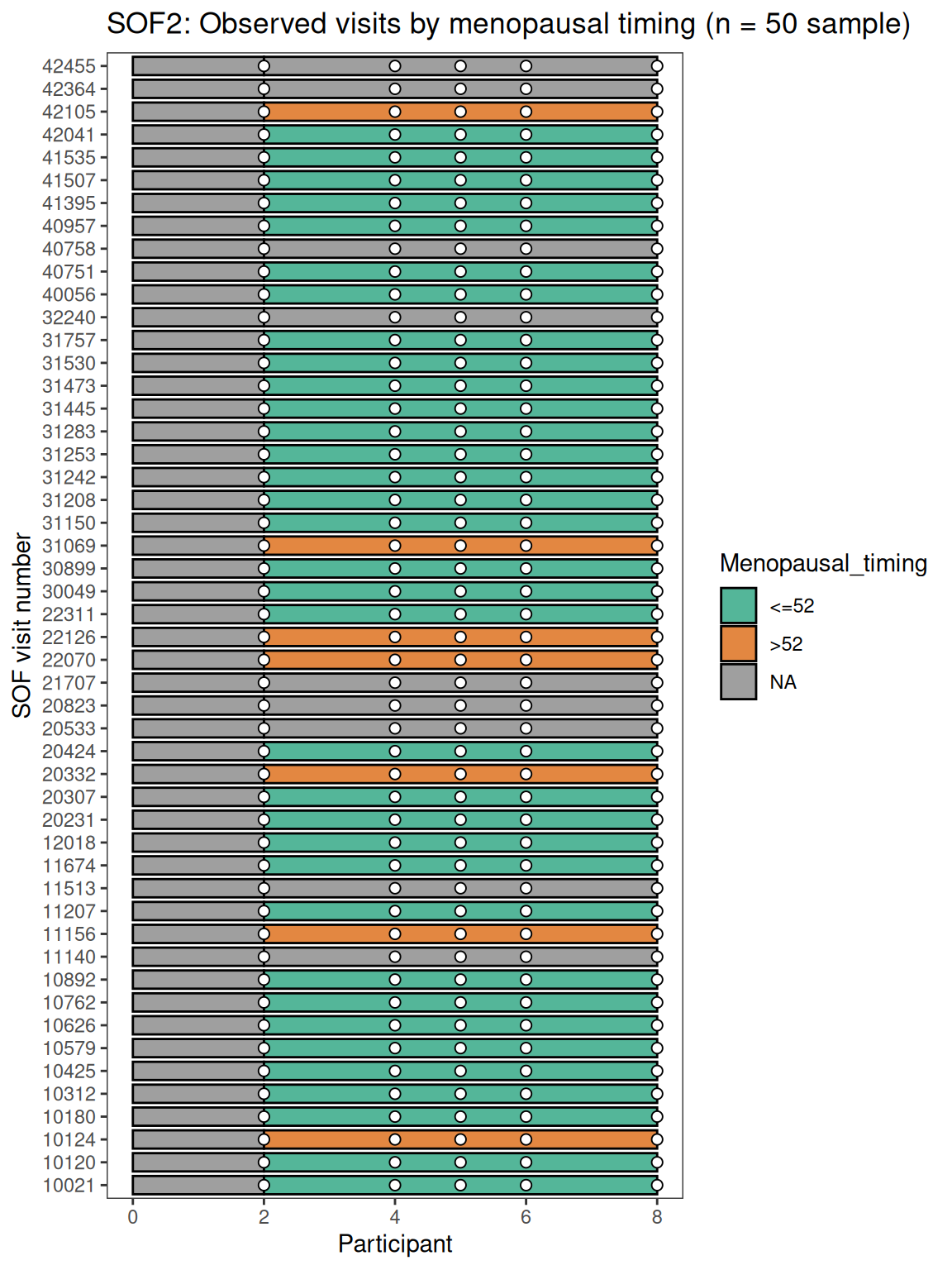
The swimmer plot below shows visit attendance for a random sample of 50 participants, colored by whether menopause occurred after age 52, with a dot at each observed visit.
set.seed(42)
dat_full <- as.data.frame(dat)
ids_sub <- sample(unique(dat_full$id), 50)
dat_sub <- dat_full[dat_full$id %in% ids_sub, ]

dat_ends <- aggregate(visit ~ id, data = dat_sub, FUN = max)
names(dat_ends)[2] <- "last_visit"
dat_starts <- aggregate(visit ~ id, data = dat_sub, FUN = min)
names(dat_starts)[2] <- "first_visit"
dat_sum <- merge(dat_ends, dat_starts, by = "id")

first_obs <- dat_full[!duplicated(dat_full$id), c("id", "meno_ov_52")]
dat_sum <- merge(dat_sum, first_obs, by = "id")
dat_sum$Menopausal_timing <- factor(
  dat_sum$meno_ov_52,
  levels = c(0, 1),
  labels = c("<=52", ">52")
)

swimplot::swimmer_plot(
  df = dat_sum, id = "id", end = "last_visit", start = "first_visit",
  name_fill = "Menopausal_timing", increasing = FALSE,
  col = "black", alpha = 0.75, width = 0.8
) +
  swimplot::swimmer_points(
    df = dat_sub, id = "id", time = "visit",
    shape = 21, size = 2, col = "black", fill = "white"
  ) +
  ggplot2::scale_fill_manual(values = c("#1b9e77", "#d95f02")) +
  ggplot2::labs(
    x = "SOF visit number",
    y = "Participant",
    title = "SOF2: Observed visits by menopausal timing (n = 50 sample)"
  )
fit <- stats::lm(formula_main, data = dat)
summary(fit)
#>
#> Call:
#> stats::lm(formula = formula_main, data = dat)
#>
#> Residuals:
#>      Min       1Q   Median       3Q      Max
#> -0.34948 -0.01330  0.00108  0.01724  0.80031
#>
#> Coefficients:
#>               Estimate Std. Error t value Pr(>|t|)
#> (Intercept) -6.137e-03  2.120e-03  -2.895  0.00380 **
#> base_totbmd  9.761e-01  2.416e-03 404.067  < 2e-16 ***
#> bmi          1.625e-03  6.454e-05  25.182  < 2e-16 ***
#> visit_spl1  -8.992e-03  3.083e-04 -29.167  < 2e-16 ***
#> visit_spl2   1.208e-03  4.383e-04   2.756  0.00585 **
#> meno_ov_52  -2.301e-04  6.824e-04  -0.337  0.73593
#> ---
#> Signif. codes:  0 '***' 0.001 '**' 0.01 '*' 0.05 '.' 0.1 ' ' 1
#>
#> Residual standard error: 0.03983 on 21349 degrees of freedom
#>   (21595 observations deleted due to missingness)
#> Multiple R-squared:  0.9086, Adjusted R-squared:  0.9086
#> F-statistic: 4.245e+04 on 5 and 21349 DF, p-value: < 2.2e-16fit_data <- data.frame(
fitted = stats::fitted(fit),
residuals = stats::residuals(fit)
)
ggplot2::ggplot(fit_data, ggplot2::aes(x = fitted, y = residuals)) +
ggplot2::geom_point(alpha = 0.2, size = 0.8) +
ggplot2::geom_hline(yintercept = 0, linetype = "dashed", color = "#d95f02") +
ggplot2::labs(
title = "Residuals vs fitted",
x = "Fitted total BMD",
y = "Residuals"
) +
ggplot2::theme_minimal()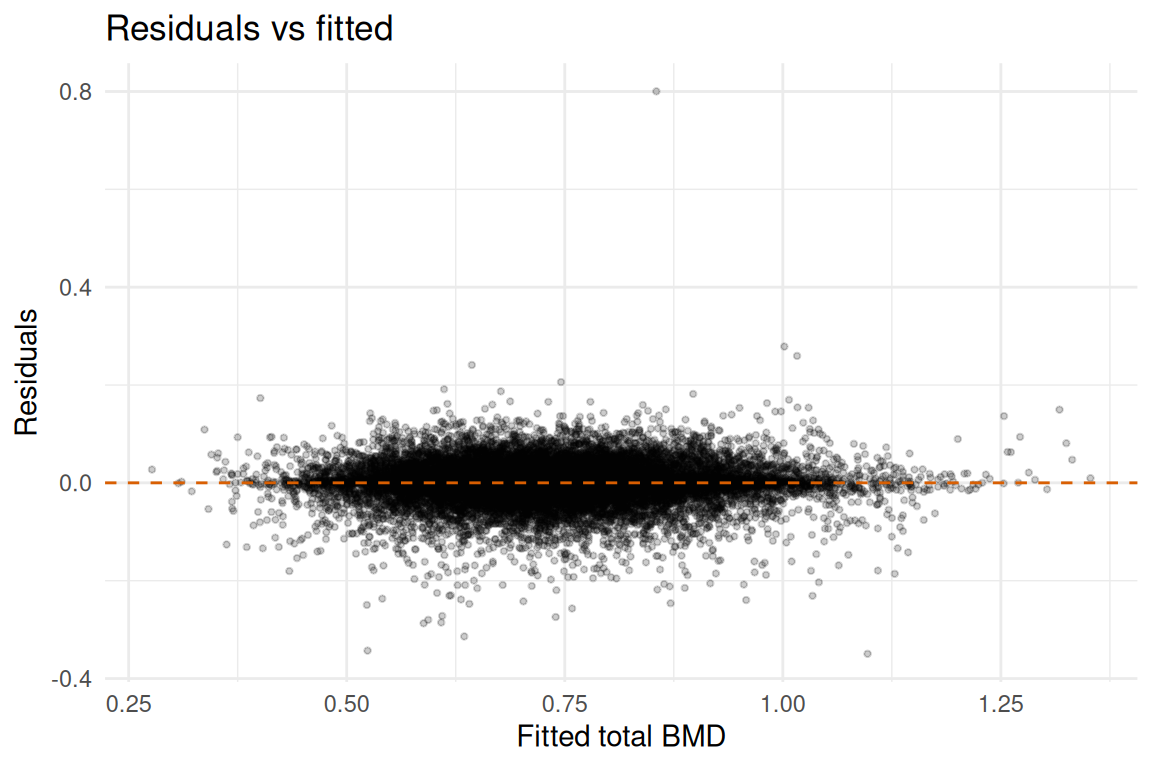
ci <- stats::confint(fit)
coefs <- summary(fit)$coefficients
data.frame(
  term = rownames(coefs),
  estimate = coefs[, "Estimate"],
  conf_low = ci[, 1],
  conf_high = ci[, 2],
  p_value = coefs[, "Pr(>|t|)"]
)
#>                    term      estimate      conf_low    conf_high       p_value
#> (Intercept) (Intercept) -0.0061370455 -0.0102928028 -0.001981288  3.800804e-03
#> base_totbmd base_totbmd  0.9760833522  0.9713485026  0.980818202  0.000000e+00
#> bmi                 bmi  0.0016253073  0.0014987979  0.001751817 6.524051e-138
#> visit_spl1   visit_spl1 -0.0089915368 -0.0095957915 -0.008387282 2.017058e-183
#> visit_spl2   visit_spl2  0.0012079485  0.0003488814  0.002067015  5.854576e-03
#> meno_ov_52 meno_ov_52 -0.0002301258 -0.0015675940 0.001107342 7.359303e-01Baseline BMD is the strongest predictor of total BMD at each subsequent visit, reflecting the high autocorrelation of bone density over time (RMB2e Ch. 7). The spline terms for visit capture the nonlinear shape of population-average BMD change. Women with late menopause (after age 52) tend to have higher BMD throughout follow-up, consistent with a longer period of estrogen exposure before the onset of accelerated bone loss. This marginal model ignores within-subject correlation; proper inference for longitudinal outcomes requires mixed-effects or GEE approaches as developed more fully in RMB2e Chapter 7.