Figure 4.1 data

This article uses the figure4_1 dataset to illustrate polynomial regression and the importance of allowing nonlinear predictor-outcome relationships, as introduced in RMB2e Chapter 4.

1 Introduction

Simple linear regression assumes that the outcome changes at a constant rate per unit increase in the predictor. When the true relationship is curved, fitting a linear model yields biased estimates and poor predictions. Polynomial regression addresses this by including higher-order terms (e.g., \(x^2\)) in the linear predictor. The figure4_1 dataset contains only the squared predictor term x2, making it a compact teaching dataset for demonstrating the quadratic model form (RMB2e Ch. 4).

data(rmb_datasets, package = "rmb")
rmb_datasets$study_design[rmb_datasets$object == "figure4_1"]
#> [1] "Illustrative teaching dataset used for model-form and linearity examples in Chapter 4."

Can a polynomial regression model better fit a nonlinear data pattern compared to a simple linear model?

1.1 Causal assumptions

set.seed(42)
dag <- ggdag::dagify(
  y ~ x + x_sq,
  labels = c(
    y = "Outcome y",
    x = "Predictor x",
    x_sq = "x squared"
  ),
  exposure = "x",
  outcome = "y"
)
ggdag::ggdag(dag, use_labels = "label", text = FALSE) +
  ggdag::theme_dag_blank() +
  ggplot2::labs(title = "Figure 4.1: Causal DAG")

2 Methods

2.1 Study sample

data(figure4_1, package = "rmb")
dat <- figure4_1
dim(dat)
#> [1] 8 1
summary(dat)
#>        x2      
#>  Min.   :1.00  
#>  1st Qu.:2.75  
#>  Median :4.50  
#>  Mean   :4.50  
#>  3rd Qu.:6.25  
#>  Max.   :8.00

2.2 Statistical analysis

Because the dataset contains only the squared predictor x2 (n = 8), we reconstruct x = sqrt(x2) and simulate a noisy outcome to illustrate fitting both a linear and a quadratic model. A simulated outcome with a mild negative quadratic component demonstrates how polynomial regression compares to simple linear regression on residual diagnostics (RMB2e Ch. 4).

set.seed(42)
x <- sqrt(dat$x2)
y <- 2 + 1.5 * x - 0.1 * x^2 + stats::rnorm(8, 0, 0.5)
demo_df <- data.frame(x = x, x2 = dat$x2, y = y)

formula_linear <- y ~ x
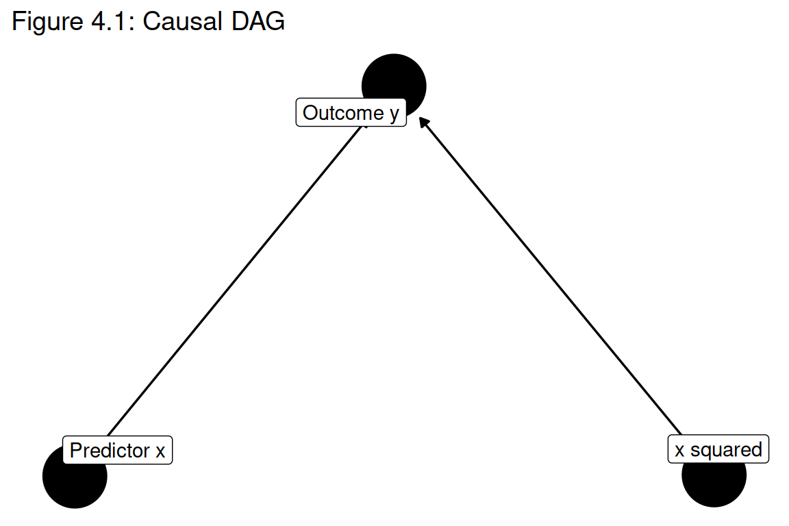
formula_quad <- y ~ x + x2

list(linear = formula_linear, quadratic = formula_quad)
#> $linear
#> y ~ x
#> 
#> $quadratic
#> y ~ x + x2

3 Results

3.1 Descriptive statistics

summary(demo_df)
#>        x               x2             y        
#>  Min.   :1.000   Min.   :1.00   Min.   :3.639  
#>  1st Qu.:1.653   1st Qu.:2.75   1st Qu.:4.381  
#>  Median :2.118   Median :4.50   Median :4.969  
#>  Mean   :2.038   Mean   :4.50   Mean   :4.827  
#>  3rd Qu.:2.499   3rd Qu.:6.25   3rd Qu.:5.141  
#>  Max.   :2.828   Max.   :8.00   Max.   :6.024
with(demo_df, cor(y, x))
#> [1] 0.8838948
with(demo_df, cor(y, x2))
#> [1] 0.8888958

ggplot2::ggplot(demo_df, ggplot2::aes(x = x, y = y)) +
  ggplot2::geom_point(color = "#1b9e77", size = 3) +
  ggplot2::labs(
    title = "Figure 4.1: Illustrative polynomial regression data",
    x = "x (sqrt of x2)",
    y = "y (simulated outcome)"
  ) +
  ggplot2::theme_minimal()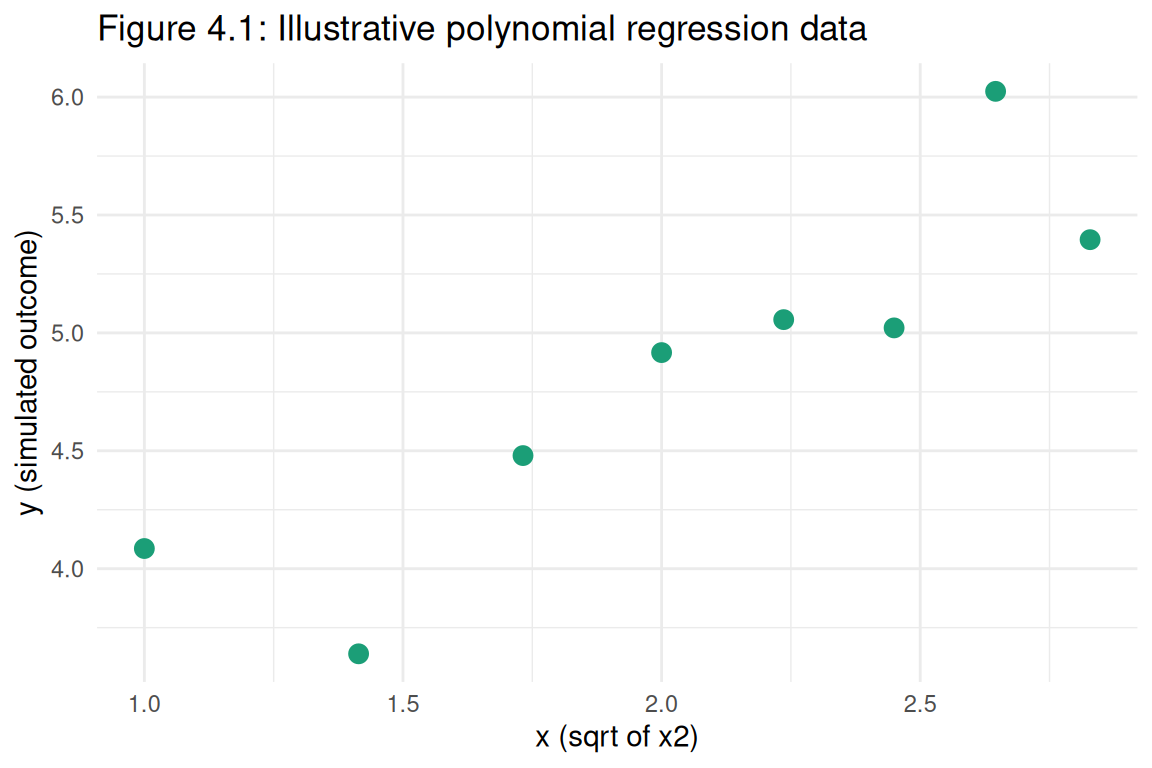

x_seq <- seq(min(demo_df$x), max(demo_df$x), length.out = 100)

3.2 Model estimates

fit_lin <- stats::lm(formula_linear, data = demo_df)
fit_quad <- stats::lm(formula_quad, data = demo_df)

summary(fit_lin)
#> 
#> Call:
#> stats::lm(formula = formula_linear, data = demo_df)
#> 
#> Residuals:
#>     Min      1Q  Median      3Q     Max 
#> -0.5300 -0.2462 -0.0021  0.1855  0.5564 
#> 
#> Coefficients:
#>             Estimate Std. Error t value Pr(>|t|)   
#> (Intercept)   2.6772     0.4834   5.539  0.00146 **
#> x             1.0548     0.2279   4.629  0.00358 **
#> ---
#> Signif. codes:  0 '***' 0.001 '**' 0.01 '*' 0.05 '.' 0.1 ' ' 1
#> 
#> Residual standard error: 0.3788 on 6 degrees of freedom
#> Multiple R-squared:  0.7813, Adjusted R-squared:  0.7448 
#> F-statistic: 21.43 on 1 and 6 DF,  p-value: 0.00358
summary(fit_quad)
#> 
#> Call:
#> stats::lm(formula = formula_quad, data = demo_df)
#> 
#> Residuals:
#>        1        2        3        4        5        6        7        8 
#>  0.24318 -0.51031  0.04434  0.20598  0.07756 -0.22080  0.52286 -0.36282 
#> attr(,"format.stata")
#> [1] "%9.0g"
#> attr(,"label")
#> [1] "Variable description not provided in source metadata."
#> 
#> Coefficients:
#>             Estimate Std. Error t value Pr(>|t|)  
#> (Intercept)   3.4078     1.6190   2.105   0.0892 .
#> x             0.2176     1.7745   0.123   0.9072  
#> x2            0.2169     0.4552   0.476   0.6539  
#> ---
#> Signif. codes:  0 '***' 0.001 '**' 0.01 '*' 0.05 '.' 0.1 ' ' 1
#> 
#> Residual standard error: 0.4059 on 5 degrees of freedom
#> Multiple R-squared:  0.7908, Adjusted R-squared:  0.7071 
#> F-statistic: 9.448 on 2 and 5 DF,  p-value: 0.02003

3.3 Model diagnostics

fit_data_lin <- data.frame(
  fitted = stats::fitted(fit_lin),
  residuals = stats::residuals(fit_lin),
  model = "Linear"
)
fit_data_quad <- data.frame(
  fitted = stats::fitted(fit_quad),
  residuals = stats::residuals(fit_quad),
  model = "Quadratic"
)

ggplot2::ggplot(fit_data_lin, ggplot2::aes(x = fitted, y = residuals)) +
  ggplot2::geom_point() +
  ggplot2::geom_hline(yintercept = 0, linetype = "dashed", color = "red") +
  ggplot2::geom_smooth(se = FALSE, color = "blue") +
  ggplot2::labs(
    title = "Linear model residuals",
    x = "Fitted values",
    y = "Residuals"
  ) +
  ggplot2::theme_minimal()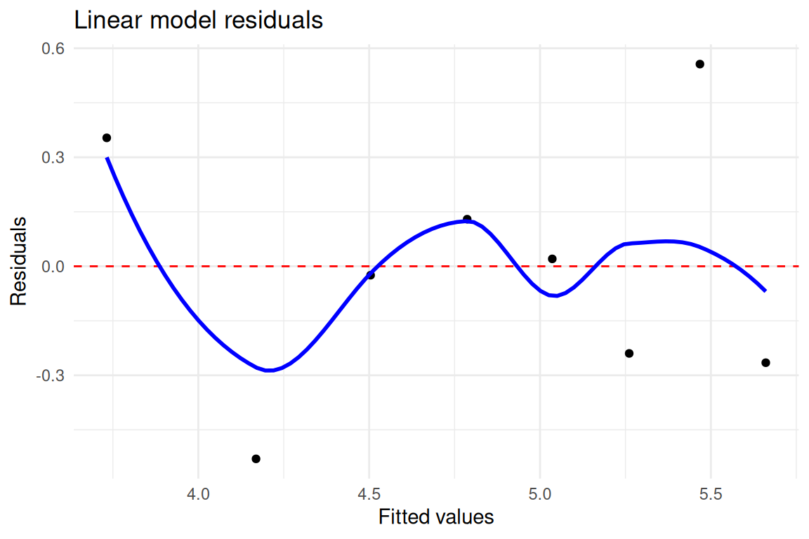

ggplot2::ggplot(fit_data_quad, ggplot2::aes(x = fitted, y = residuals)) +
  ggplot2::geom_point() +
  ggplot2::geom_hline(yintercept = 0, linetype = "dashed", color = "red") +
  ggplot2::geom_smooth(se = FALSE, color = "blue") +
  ggplot2::labs(
    title = "Quadratic model residuals",
    x = "Fitted values",
    y = "Residuals"
  ) +
  ggplot2::theme_minimal()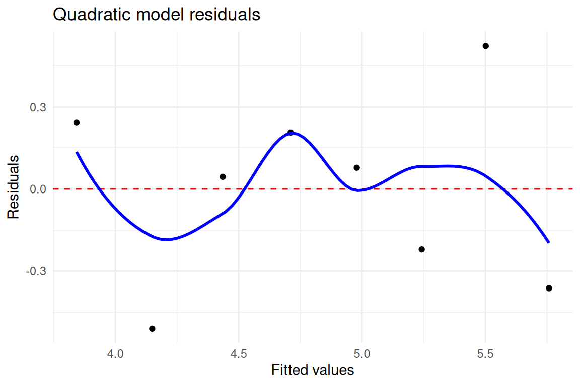

3.4 Inference

ci_lin <- stats::confint(fit_lin)
ci_quad <- stats::confint(fit_quad)

data.frame(
  model = c("linear x", "quad x", "quad x2"),
  estimate = c(
    stats::coef(fit_lin)["x"],
    stats::coef(fit_quad)["x"],
    stats::coef(fit_quad)["x2"]
  ),
  conf_low = c(ci_lin["x", 1], ci_quad["x", 1], ci_quad["x2", 1]),
  conf_high = c(ci_lin["x", 2], ci_quad["x", 2], ci_quad["x2", 2])
)
#>      model  estimate   conf_low conf_high
#> 1 linear x 1.0548364  0.4972895  1.612383
#> 2   quad x 0.2176070 -4.3439333  4.779147
#> 3  quad x2 0.2168509 -0.9533999  1.387102

4 Discussion

Including the squared term x2 changes the estimated slope for x compared to the linear-only model, illustrating how omitting a curved component can distort the linear coefficient (RMB2e Ch. 4). The residual plots for the quadratic model show less systematic pattern than those for the linear model, suggesting better fit. This toy example motivates the model-checking workflow of Chapter 4: plotting residuals against fitted values is a key diagnostic for detecting nonlinearity that a simple linear term cannot capture.

5 Source

• UCSF Regression Methods companion data: figure 4.1 illustrative dataset (RMB2e Chapter 4).
• Book: Vittinghoff E, Glidden DV, Shiboski SC, McCulloch CE (2012). Regression Methods in Biostatistics (2nd edition).