PBC data

This article fits a Cox proportional hazards model to the primary biliary cirrhosis (PBC) trial data, identifying clinical predictors of mortality as described in RMB2e Chapter 6.

1 Introduction

Primary biliary cirrhosis (PBC) is a chronic autoimmune cholestatic liver disease that, if untreated, progresses to cirrhosis and liver failure. Dickson and colleagues (1989) analyzed data from a Mayo Clinic placebo-controlled trial of D-penicillamine in 312 PBC patients, establishing serum bilirubin, albumin, and prothrombin time as the dominant predictors of survival. Log-transforming these biomarkers improves linearity of the log-hazard relationship and is standard practice in PBC prognostic modeling (RMB2e Ch. 6).

Code

data(rmb_datasets, package = "rmb")
rmb_datasets$study_design[rmb_datasets$object == "pbc"]
#> [1] "Placebo-controlled clinical trial cohort in primary biliary cirrhosis (D-penicillamine)."

Is higher log-bilirubin associated with shorter survival in PBC after adjustment for log-albumin, log-prothrombin time, age, and edema status?

1.1 Causal assumptions

Code

set.seed(42)
dag <- ggdag::dagify(
  surv ~ bili + albu + prot + age + edema,
  labels = c(
    surv = "Survival",
    bili = "Log bilirubin",
    albu = "Log albumin",
    prot = "Prothrombin time",
    age = "Age",
    edema = "Edema"
  ),
  exposure = "bili",
  outcome = "surv"
)
ggdag::ggdag(dag, use_labels = "label", text = FALSE) +
  ggdag::theme_dag_blank() +
  ggplot2::labs(title = "PBC: Causal DAG")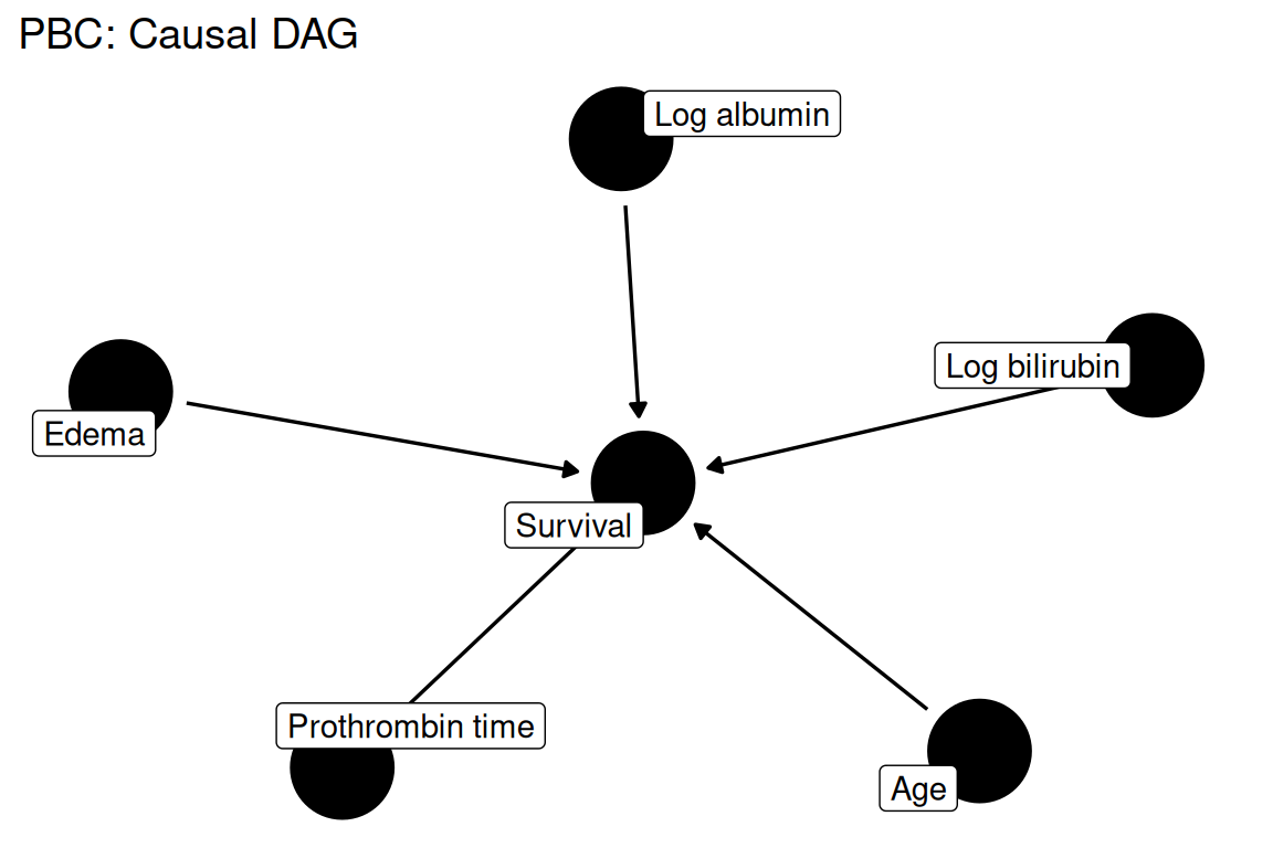

Figure 1: Directed acyclic graph for predictors of PBC survival risk.

2 Methods

2.1 Study sample

Code

data(pbc, package = "rmb")
dat <- pbc
dat$status <- as.integer(unclass(dat$status))
dim(dat)
#> [1] 312  23
summary(haven::zap_labels(dat[c("years", "status", "rx", "logbili", "logalbu", "logprot", "age", "edema")]))
#>      years             status             rx            logbili       
#>  Min.   : 0.1123   Min.   :0.0000   Min.   :0.0000   Min.   :-1.2040  
#>  1st Qu.: 3.2608   1st Qu.:0.0000   1st Qu.:0.0000   1st Qu.:-0.2231  
#>  Median : 5.0363   Median :0.0000   Median :0.0000   Median : 0.2994  
#>  Mean   : 5.4931   Mean   :0.4006   Mean   :0.4936   Mean   : 0.5757  
#>  3rd Qu.: 7.3847   3rd Qu.:1.0000   3rd Qu.:1.0000   3rd Qu.: 1.2310  
#>  Max.   :12.4736   Max.   :1.0000   Max.   :1.0000   Max.   : 3.3322  
#>     logalbu          logprot           age            edema       
#>  Min.   :0.6729   Min.   :2.197   Min.   :26.28   Min.   :0.0000  
#>  1st Qu.:1.1969   1st Qu.:2.303   1st Qu.:42.24   1st Qu.:0.0000  
#>  Median :1.2669   Median :2.361   Median :49.79   Median :0.0000  
#>  Mean   :1.2508   Mean   :2.369   Mean   :50.02   Mean   :0.1571  
#>  3rd Qu.:1.3350   3rd Qu.:2.407   3rd Qu.:56.71   3rd Qu.:0.0000  
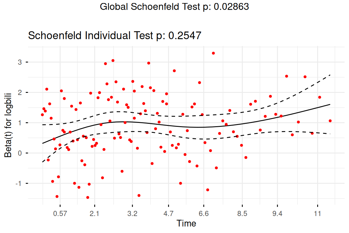
#>  Max.   :1.5347   Max.   :2.839   Max.   :78.44   Max.   :1.0000

2.2 Statistical analysis

A Cox proportional hazards model is fitted with death (status == 1) as the event, using log-transformed bilirubin, albumin, and prothrombin time plus age and edema as predictors (RMB2e Ch. 6 / Dickson 1989). The proportional hazards assumption is checked with scaled Schoenfeld residuals.

Code

formula_main <- survival::Surv(years, status == 1) ~ logbili + logalbu + logprot + age + edema
formula_main
#> survival::Surv(years, status == 1) ~ logbili + logalbu + logprot + 
#>     age + edema

3 Results

3.1 Descriptive statistics

Code

with(dat, table(status))
#> status
#>   0   1 
#> 187 125
with(dat, table(rx, status))
#>    status
#> rx   0  1
#>   0 93 65
#>   1 94 60
summary(haven::zap_labels(dat[c("logbili", "logalbu", "logprot", "age")]))
#>     logbili           logalbu          logprot           age       
#>  Min.   :-1.2040   Min.   :0.6729   Min.   :2.197   Min.   :26.28  
#>  1st Qu.:-0.2231   1st Qu.:1.1969   1st Qu.:2.303   1st Qu.:42.24  
#>  Median : 0.2994   Median :1.2669   Median :2.361   Median :49.79  
#>  Mean   : 0.5757   Mean   :1.2508   Mean   :2.369   Mean   :50.02  
#>  3rd Qu.: 1.2310   3rd Qu.:1.3350   3rd Qu.:2.407   3rd Qu.:56.71  
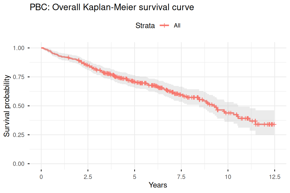
#>  Max.   : 3.3322   Max.   :1.5347   Max.   :2.839   Max.   :78.44

Code

km_all <- survival::survfit(survival::Surv(years, status == 1) ~ 1, data = dat)

survminer::ggsurvplot(
  km_all,
  data = dat,
  title = "PBC: Overall Kaplan-Meier survival curve",
  xlab = "Years",
  ylab = "Survival probability",
  ggtheme = ggplot2::theme_minimal(),
  conf.int = TRUE,
  censor = TRUE
)

Figure 2: Overall Kaplan-Meier survival curve for the PBC study cohort.

3.2 Model estimates

Code

fit <- survival::coxph(formula_main, data = dat, ties = "breslow")
summary(fit)
#> Call:
#> survival::coxph(formula = formula_main, data = dat, ties = "breslow")
#> 
#>   n= 312, number of events= 125 
#> 
#>              coef exp(coef)  se(coef)      z Pr(>|z|)    
#> logbili  0.893670  2.444082  0.098024  9.117  < 2e-16 ***
#> logalbu -3.222238  0.039866  0.707486 -4.554 5.25e-06 ***
#> logprot  3.237471 25.469238  0.998051  3.244 0.001179 ** 
#> age      0.032652  1.033191  0.008627  3.785 0.000154 ***
#> edema    0.399062  1.490426  0.221498  1.802 0.071601 .  
#> ---
#> Signif. codes:  0 '***' 0.001 '**' 0.01 '*' 0.05 '.' 0.1 ' ' 1
#> 
#>         exp(coef) exp(-coef) lower .95 upper .95
#> logbili   2.44408    0.40915  2.016868    2.9618
#> logalbu   0.03987   25.08420  0.009963    0.1595
#> logprot  25.46924    0.03926  3.601419  180.1185
#> age       1.03319    0.96788  1.015867    1.0508
#> edema     1.49043    0.67095  0.965541    2.3006
#> 
#> Concordance= 0.843  (se = 0.02 )
#> Likelihood ratio test= 195.7  on 5 df,   p=<2e-16
#> Wald test            = 192.5  on 5 df,   p=<2e-16
#> Score (logrank) test = 251.1  on 5 df,   p=<2e-16

3.3 Model diagnostics

Code

ph_test <- survival::cox.zph(fit)
ph_test
#>         chisq df     p
#> logbili  1.30  1 0.255
#> logalbu  0.39  1 0.532
#> logprot  5.99  1 0.014
#> age      0.85  1 0.356
#> edema    6.51  1 0.011
#> GLOBAL  12.49  5 0.029

survminer::ggcoxzph(
  ph_test,
  var = "logbili",
  ggtheme = ggplot2::theme_minimal()
)

Figure 3: Scaled Schoenfeld residual plot for the log-bilirubin covariate effect.

3.4 Inference

Code

hr <- exp(stats::coef(fit))
ci <- exp(stats::confint(fit))
knitr::kable(data.frame(
  term = names(hr),
  hazard_ratio = unname(hr),
  conf_low = ci[, 1],
  conf_high = ci[, 2],
  p_value = summary(fit)$coefficients[, "Pr(>|z|)"]
), digits = 3)

Table 1: Cox model hazard-ratio estimates with confidence intervals for PBC.

	term	hazard_ratio	conf_low	conf_high	p_value
logbili	logbili	2.444	2.017	2.962	0.000
logalbu	logalbu	0.040	0.010	0.160	0.000
logprot	logprot	25.469	3.601	180.118	0.001
age	age	1.033	1.016	1.051	0.000
edema	edema	1.490	0.966	2.301	0.072

4 Discussion

Log-bilirubin, log-albumin, log-prothrombin time, age, and edema are all strongly associated with mortality risk in PBC, confirming the Mayo Clinic prognostic model reported by Dickson et al. (1989) and discussed in RMB2e Chapter 6. Bilirubin shows the largest hazard ratio, consistent with its role as the primary index of hepatic synthetic dysfunction in cholestatic disease. The Schoenfeld residual plots should be inspected to confirm that the proportional hazards assumption is tenable for each predictor across the observation period.

5 Source

Dickson ER et al. (1989). Prognosis in primary biliary cirrhosis: model for decision making. Hepatology, 10(1), 1–7.
UCSF Regression Methods companion data: https://regression.ucsf.edu/sites/g/files/tkssra16191/files/wysiwyg/home/data/pbc.dta
Book: Vittinghoff E, Glidden DV, Shiboski SC, McCulloch CE (2012). Regression Methods in Biostatistics (2nd edition).