Code
data(rmb_datasets, package = "rmb")
rmb_datasets$study_design[rmb_datasets$object == "wcgs"]
#> [1] "Prospective epidemiologic cohort of middle-aged men studying Type A behavior and CHD risk."This article reproduces key WCGS analyses from RMB2e Chapters 2, 3, and 5, modelling coronary heart disease risk from standard cardiovascular risk factors.
The Western Collaborative Group Study (WCGS) enrolled approximately 3,500 employed men aged 39–59 in California in 1960–1961 and followed them for roughly 8.5 years to study coronary heart disease (CHD) incidence. WCGS was among the first prospective cohort studies to establish the Type A behavior pattern as a CHD risk factor alongside classical predictors such as age, serum cholesterol, and blood pressure. These data illustrate the logistic regression framework for binary outcomes (RMB2e Chapter 5, pp. 171–177).
data(rmb_datasets, package = "rmb")
rmb_datasets$study_design[rmb_datasets$object == "wcgs"]
#> [1] "Prospective epidemiologic cohort of middle-aged men studying Type A behavior and CHD risk."How are established cardiovascular risk factors—age, cholesterol, systolic blood pressure, BMI, smoking, and behavior pattern—jointly associated with CHD incidence in WCGS men?
set.seed(42)
dag <- ggdag::dagify(
  chd ~ age + chol + sbp + bmi + smoke + beh,
  smoke ~ beh,
  sbp ~ age,
  chol ~ age,
  labels = c(
    chd = "CHD by follow-up",
    age = "Age",
    chol = "Cholesterol",
    sbp = "Systolic BP",
    bmi = "BMI",
    smoke = "Smoking",
    beh = "Behavior pattern"
  ),
  exposure = "beh",
  outcome = "chd"
)
ggdag::ggdag(dag, use_labels = "label", text = FALSE) +
  ggdag::theme_dag_blank() +
  ggplot2::labs(title = "WCGS: Causal DAG")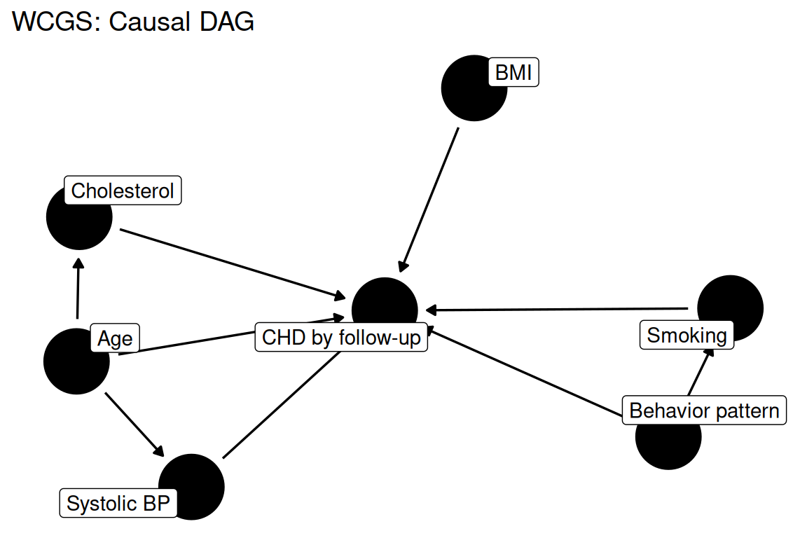
data(wcgs, package = "rmb")
dat <- haven::zap_labels(wcgs)
dim(dat)
#> [1] 3154   22
summary(dat[c("sbp", "weight", "chd69", "age", "chol", "bmi", "smoke", "behpat")])
#>       sbp            weight        chd69              age
#>  Min.   : 98.0   Min.   : 78   Min.   :0.00000   Min.   :39.00
#>  1st Qu.:120.0   1st Qu.:155   1st Qu.:0.00000   1st Qu.:42.00
#>  Median :126.0   Median :170   Median :0.00000   Median :45.00
#>  Mean   :128.6   Mean   :170   Mean   :0.08148   Mean   :46.28
#>  3rd Qu.:136.0   3rd Qu.:182   3rd Qu.:0.00000   3rd Qu.:50.00
#>  Max.   :230.0   Max.   :320   Max.   :1.00000   Max.   :59.00
#>
#>       chol            bmi            smoke            behpat
#>  Min.   :103.0   Min.   :11.19   Min.   :0.0000   Min.   :1.000
#>  1st Qu.:197.2   1st Qu.:22.96   1st Qu.:0.0000   1st Qu.:2.000
#>  Median :223.0   Median :24.39   Median :0.0000   Median :2.000
#>  Mean   :226.4   Mean   :24.52   Mean   :0.4762   Mean   :2.523
#>  3rd Qu.:253.0   3rd Qu.:25.84   3rd Qu.:1.0000   3rd Qu.:3.000
#>  Max.   :645.0   Max.   :38.95   Max.   :1.0000   Max.   :4.000
#> NAs :12Following RMB2e Chapter 5 (pp. 171, 175), two logistic regression models are fitted on a cleaned sample (excluding one outlier with cholesterol ≥ 645 mg/dL): a base model with five standard risk factors, and an extended model adding categorical behavior pattern to test its independent contribution via a likelihood-ratio test.
ana <- subset(dat, chol < 645)
ana$age_10 <- ana$age / 10
ana$chol_50 <- ana$chol / 50
ana$sbp_50 <- ana$sbp / 50
ana$bmi_10 <- ana$bmi / 10
ana$smoke <- factor(ana$smoke)
ana$behpat <- factor(ana$behpat)

formula_base <- chd69 ~ age_10 + chol_50 + sbp_50 + bmi_10 + smoke
formula_behpat <- update(formula_base, . ~ . + behpat)

list(base = formula_base, with_behpat = formula_behpat)
#> $base
#> chd69 ~ age_10 + chol_50 + sbp_50 + bmi_10 + smoke
#>
#> $with_behpat
#> chd69 ~ age_10 + chol_50 + sbp_50 + bmi_10 + smoke + behpatsummary(dat$sbp)
#> Min. 1st Qu. Median Mean 3rd Qu. Max.
#> 98.0 120.0 126.0 128.6 136.0 230.0
summary(dat$weight)
#> Min. 1st Qu. Median Mean 3rd Qu. Max.
#> 78 155 170 170 182 320
with(dat, cor(sbp, weight, use = "complete.obs"))
#> [1] 0.2532496
with(dat, table(behpat, useNA = "ifany"))
#> behpat
#> 1 2 3 4
#> 264 1325 1216 349
with(dat, prop.table(table(chd69)))
#> chd69
#> 0 1
#> 0.91851617 0.08148383ggplot2::ggplot(dat, ggplot2::aes(x = sbp)) +
ggplot2::geom_histogram(bins = 15, fill = "grey85", color = "white") +
ggplot2::labs(
title = "WCGS systolic blood pressure",
x = "SBP (mmHg)",
y = "Frequency"
) +
ggplot2::theme_minimal()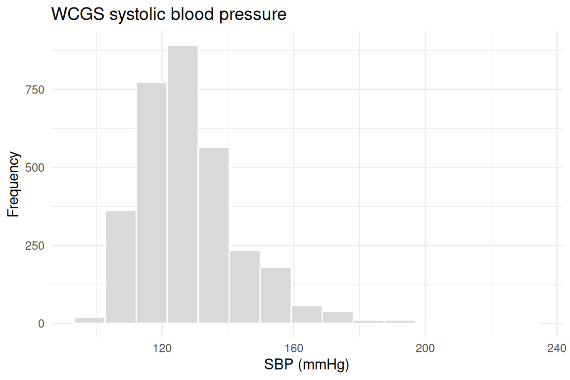
fit_base <- stats::glm(formula_base, data = ana, family = stats::binomial())
fit_behpat <- stats::glm(formula_behpat, data = ana, family = stats::binomial())

summary(fit_base)
#>
#> Call:
#> stats::glm(formula = formula_base, family = stats::binomial(),
#>     data = ana)
#>
#> Coefficients:
#>              Estimate Std. Error z value Pr(>|z|)
#> (Intercept) -12.31099    0.97726 -12.598  < 2e-16 ***
#> age_10        0.64448    0.11907   5.412 6.22e-08 ***
#> chol_50       0.53706    0.07586   7.079 1.45e-12 ***
#> sbp_50        0.96469    0.20454   4.716 2.40e-06 ***
#> bmi_10        0.57436    0.26355   2.179   0.0293 *
#> smoke1        0.63448    0.14018   4.526 6.01e-06 ***
#> ---
#> Signif. codes:  0 '***' 0.001 '**' 0.01 '*' 0.05 '.' 0.1 ' ' 1
#>
#> (Dispersion parameter for binomial family taken to be 1)
#>
#>     Null deviance: 1774.2  on 3140  degrees of freedom
#> Residual deviance: 1614.4  on 3135  degrees of freedom
#> AIC: 1626.4
#>
#> Number of Fisher Scoring iterations: 6
summary(fit_behpat)
#>
#> Call:
#> stats::glm(formula = formula_behpat, family = stats::binomial(),
#>     data = ana)
#>
#> Coefficients:
#>              Estimate Std. Error z value Pr(>|z|)
#> (Intercept) -11.64889    1.01421 -11.486  < 2e-16 ***
#> age_10        0.60636    0.11990   5.057 4.25e-07 ***
#> chol_50       0.53304    0.07637   6.980 2.96e-12 ***
#> sbp_50        0.90158    0.20647   4.367 1.26e-05 ***
#> bmi_10        0.55355    0.26563   2.084  0.03717 *
#> smoke1        0.60468    0.14110   4.285 1.82e-05 ***
#> behpat2       0.06603    0.22123   0.298  0.76535
#> behpat3      -0.66522    0.24226  -2.746  0.00603 **
#> behpat4      -0.55849    0.31921  -1.750  0.08019 .
#> ---
#> Signif. codes:  0 '***' 0.001 '**' 0.01 '*' 0.05 '.' 0.1 ' ' 1
#>
#> (Dispersion parameter for binomial family taken to be 1)
#>
#>     Null deviance: 1774.2  on 3140  degrees of freedom
#> Residual deviance: 1589.6  on 3132  degrees of freedom
#> AIC: 1607.6
#>
#> Number of Fisher Scoring iterations: 6stats::anova(fit_base, fit_behpat, test = "Chisq")
#> Analysis of Deviance Table
#>
#> Model 1: chd69 ~ age_10 + chol_50 + sbp_50 + bmi_10 + smoke
#> Model 2: chd69 ~ age_10 + chol_50 + sbp_50 + bmi_10 + smoke + behpat
#> Resid. Df Resid. Dev Df Deviance Pr(>Chi)
#> 1 3135 1614.4
#> 2 3132 1589.6 3 24.765 1.729e-05 ***
#> ---
#> Signif. codes: 0 '***' 0.001 '**' 0.01 '*' 0.05 '.' 0.1 ' ' 1
pred <- stats::fitted(fit_behpat)
cut_pred <- cut(pred, breaks = stats::quantile(pred, probs = seq(0, 1, by = 0.1)), include.lowest = TRUE)
obs <- tapply(ana$chd69, cut_pred, mean)
expected_prob <- tapply(pred, cut_pred, mean)
data.frame(decile = names(obs), observed = as.numeric(obs), expected = as.numeric(expected_prob))
#> decile observed expected
#> 1 [0.00443,0.019] 0.006349206 0.01421274
#> 2 (0.019,0.0273] 0.022292994 0.02312116
#> 3 (0.0273,0.0369] 0.031847134 0.03190256
#> 4 (0.0369,0.0466] 0.028662420 0.04159867
#> 5 (0.0466,0.0586] 0.073248408 0.05257476
#> 6 (0.0586,0.0724] 0.041401274 0.06516772
#> 7 (0.0724,0.0933] 0.070063694 0.08266049
#> 8 (0.0933,0.122] 0.152866242 0.10673528
#> 9 (0.122,0.172] 0.156050955 0.14409293
#> 10 (0.172,0.555] 0.232484076 0.25317505or <- exp(stats::coef(fit_behpat))
ci <- exp(stats::confint(fit_behpat))
inf <- data.frame(
term = names(or),
odds_ratio = unname(or),
conf_low = ci[, 1],
conf_high = ci[, 2],
p_value = summary(fit_behpat)$coefficients[, "Pr(>|z|)"]
)
inf
#> term odds_ratio conf_low conf_high p_value
#> (Intercept) (Intercept) 8.728745e-06 1.169564e-06 0.0000625015 1.556790e-30
#> age_10 age_10 1.833750e+00 1.449665e+00 2.3202948959 4.254445e-07
#> chol_50 chol_50 1.704097e+00 1.467336e+00 1.9798506916 2.956099e-12
#> sbp_50 sbp_50 2.463505e+00 1.636219e+00 3.6788537152 1.262183e-05
#> bmi_10 bmi_10 1.739414e+00 1.030643e+00 2.9206747410 3.716580e-02
#> smoke1 smoke1 1.830672e+00 1.391118e+00 2.4200886806 1.823581e-05
#> behpat2 behpat2 1.068257e+00 7.013746e-01 1.6738007708 7.653499e-01
#> behpat3 behpat3 5.141593e-01 3.223790e-01 0.8357872693 6.034086e-03
#> behpat4 behpat4 5.720710e-01 3.011949e-01 1.0602818756 8.018746e-02Consistent with RMB2e Chapter 5 (pp. 171, 175–177), older age, higher cholesterol, higher systolic blood pressure, higher BMI, and smoking are each associated with increased CHD odds after mutual adjustment. Behavior pattern (Type A vs B) contributes additional independent information about CHD risk, as demonstrated by the likelihood-ratio test comparing the base and extended models. The decile calibration table confirms reasonable model fit across the risk spectrum, an important diagnostic step for logistic regression (RMB2e p. 175).