UNOS data

This article fits a Cox proportional hazards model to pediatric kidney transplant recipients in the UNOS registry, comparing post-transplant mortality between living-donor and cadaveric recipients (RMB2e Chapter 6).

1 Introduction

Kidney transplantation offers superior outcomes compared to long-term dialysis for children with end-stage renal disease. Living-donor transplants are hypothesized to have better outcomes than cadaveric transplants due to shorter cold ischemic time, better HLA matching opportunities, and planned surgery timing. The UNOS (United Network for Organ Sharing) registry provides observational data on outcomes for all US transplant recipients, enabling registry-based Cox regression adjusted for recipient and donor characteristics (RMB2e Ch. 6).

Code

data(rmb_datasets, package = "rmb")
rmb_datasets$study_design[rmb_datasets$object == "unos"]
#> [1] "Registry-based cohort of pediatric kidney transplant recipients from the UNOS database."

Is living-donor transplant associated with lower post-transplant mortality compared to cadaveric transplant in pediatric kidney recipients?

1.1 Causal assumptions

Code

set.seed(42)
dag <- ggdag::dagify(
  mort ~ txtype + age + agedon + cold + rej,
  labels = c(
    mort = "Post-transplant mortality",
    txtype = "Living vs cadaveric",
    age = "Age",
    agedon = "Donor age",
    cold = "Cold ischemic time",
    rej = "Rejection 1yr"
  ),
  exposure = "txtype",
  outcome = "mort"
)
ggdag::ggdag(dag, use_labels = "label", text = FALSE) +
  ggdag::theme_dag_blank() +
  ggplot2::labs(title = "UNOS: Causal DAG")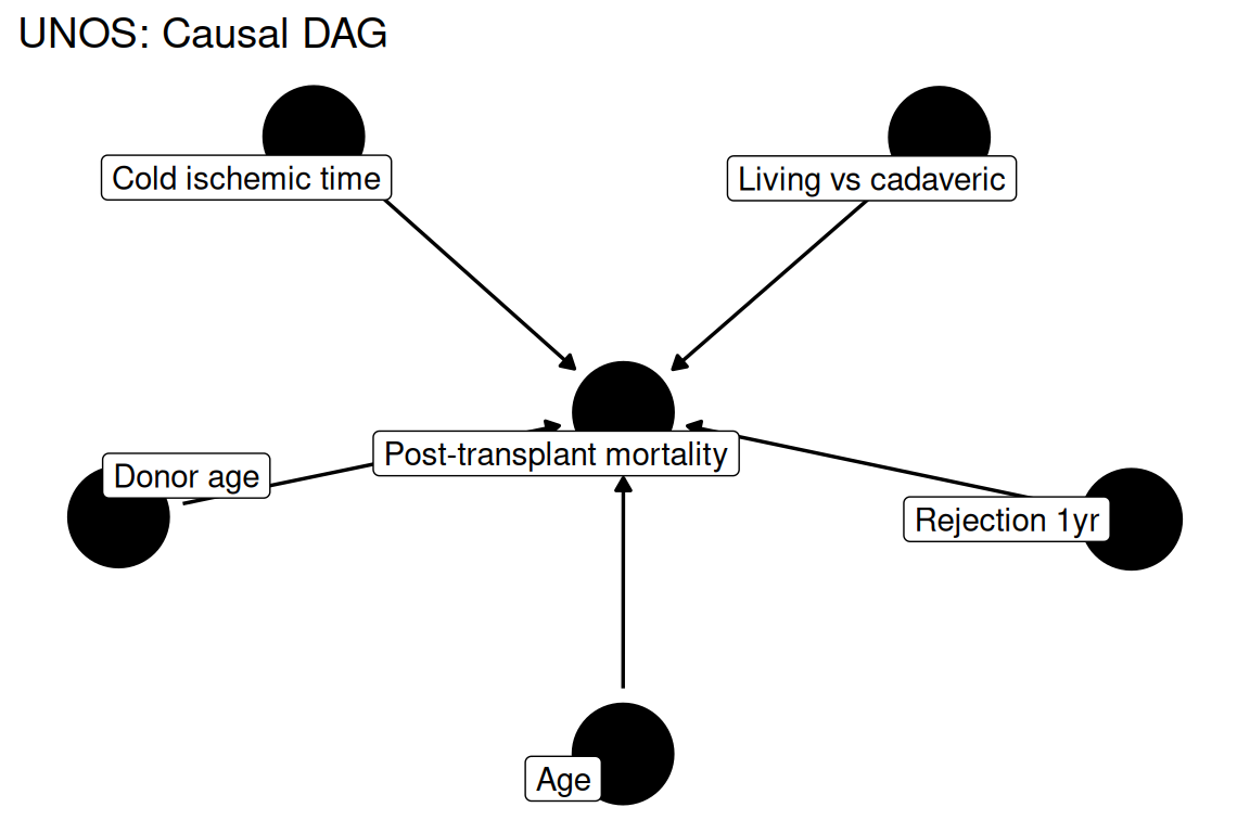

Figure 1: Directed acyclic graph for donor type and pediatric transplant mortality.

2 Methods

2.1 Study sample

Code

data(unos, package = "rmb")
dat <- unos
dim(dat)
#> [1] 9775   25
summary(haven::zap_labels(dat[c("death", "fu", "txtype", "age", "age_don", "cold_isc", "trtrej1y")]))
#>      death               fu             txtype            age       
#>  Min.   :0.00000   Min.   : 0.000   Min.   :0.0000   Min.   : 0.00  
#>  1st Qu.:0.00000   1st Qu.: 1.096   1st Qu.:0.0000   1st Qu.: 8.00  
#>  Median :0.00000   Median : 3.115   Median :0.0000   Median :13.00  
#>  Mean   :0.04757   Mean   : 3.888   Mean   :0.4734   Mean   :11.65  
#>  3rd Qu.:0.00000   3rd Qu.: 5.978   3rd Qu.:1.0000   3rd Qu.:16.00  
#>  Max.   :1.00000   Max.   :12.532   Max.   :1.0000   Max.   :18.00  
#>                                                      NAs    :9      
#>     age_don        cold_isc          trtrej1y   
#>  Min.   : 0.0   Min.   : 0.00   Length   :9775  
#>  1st Qu.:21.0   1st Qu.: 1.00   N.unique :   3  
#>  Median :33.0   Median : 7.00   N.blank  :3797  
#>  Mean   :31.3   Mean   :10.86   Min.nchar:   0  
#>  3rd Qu.:41.0   3rd Qu.:19.00   Max.nchar:   1  
#>  Max.   :73.0   Max.   :72.00                   
#>  NAs    :113    NAs    :2250

2.2 Statistical analysis

A Cox proportional hazards model is fitted with post-transplant death as the event, using follow-up time fu (years) and adjusting for transplant type, recipient age, donor age, cold ischemic time, and first-year rejection (RMB2e Ch. 6).

Code

formula_main <- survival::Surv(fu, death) ~ txtype + age + age_don + cold_isc + trtrej1y
formula_main
#> survival::Surv(fu, death) ~ txtype + age + age_don + cold_isc + 
#>     trtrej1y

3 Results

3.1 Descriptive statistics

Code

with(dat, table(txtype, death))
#>       death
#> txtype    0    1
#>      0 4971  177
#>      1 4339  288
with(dat, prop.table(table(txtype, death), margin = 1))
#>       death
#> txtype          0          1
#>      0 0.96561772 0.03438228
#>      1 0.93775665 0.06224335
with(dat, tapply(fu, txtype, summary))
#> $`0`
#>    Min. 1st Qu.  Median    Mean 3rd Qu.    Max. 
#>   0.000   1.112   3.277   4.020   6.041  12.288 
#> 
#> $`1`
#>    Min. 1st Qu.  Median    Mean 3rd Qu.    Max. 
#>   0.000   1.077   3.033   3.741   5.644  12.532

Code

dat$txtype_plot <- factor(
  dat$txtype,
  levels = c(0, 1),
  labels = c("Cadaveric", "Living donor")
)
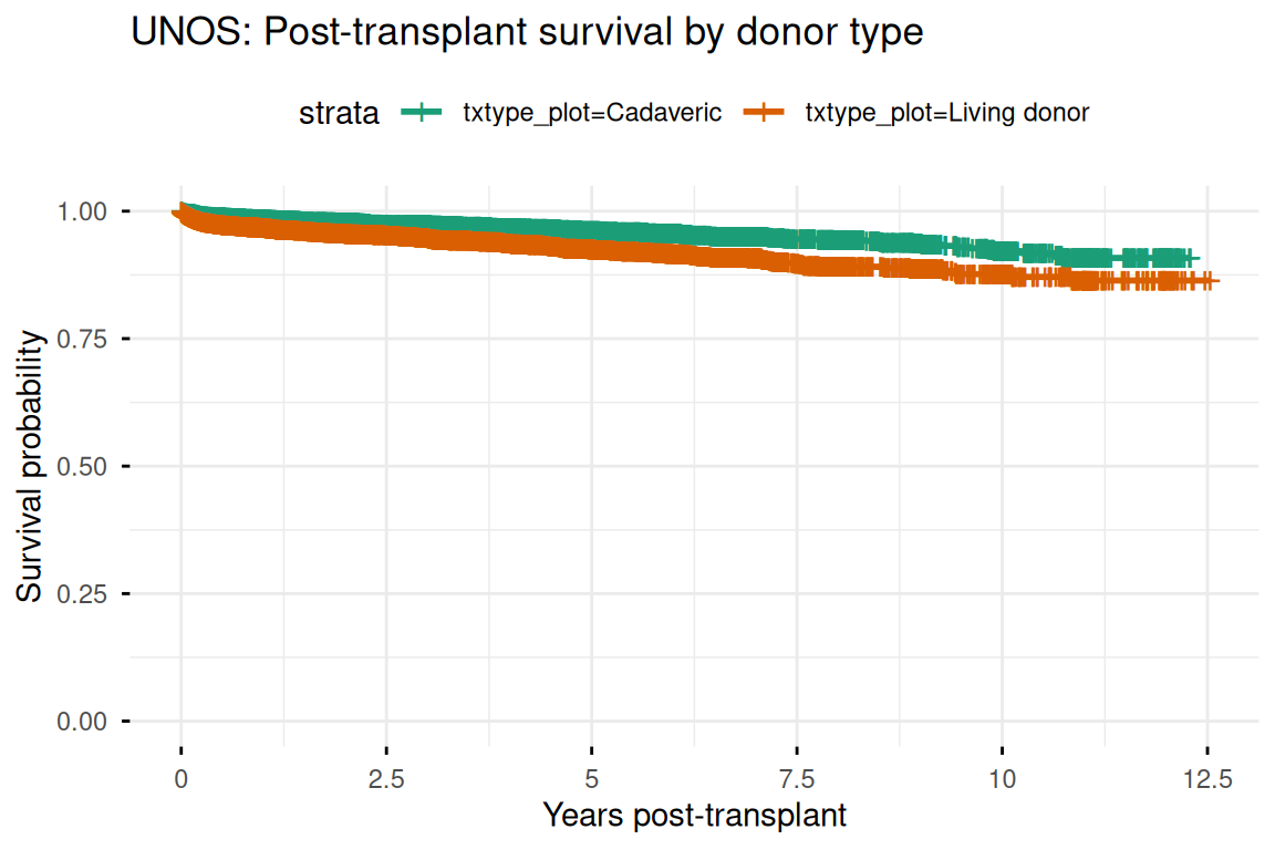
km_fit <- survival::survfit(survival::Surv(fu, death) ~ txtype_plot, data = dat)

survminer::ggsurvplot(
  km_fit,
  data = dat,
  title = "UNOS: Post-transplant survival by donor type",
  xlab = "Years post-transplant",
  ylab = "Survival probability",
  legend.title = NULL,
  ggtheme = ggplot2::theme_minimal(),
  palette = c("#1b9e77", "#d95f02"),
  conf.int = FALSE,
  censor = TRUE
)

Figure 2: Kaplan-Meier survival curves by donor type in pediatric recipients.

3.2 Model estimates

Code

fit <- survival::coxph(formula_main, data = dat, ties = "breslow")
summary(fit)
#> Call:
#> survival::coxph(formula = formula_main, data = dat, ties = "breslow")
#> 
#>   n= 7480, number of events= 356 
#>    (2295 observations deleted due to missingness)
#> 
#>                coef exp(coef)  se(coef)       z Pr(>|z|)    
#> txtype     0.427718  1.533754  0.173946   2.459   0.0139 *  
#> age       -0.024218  0.976073  0.010121  -2.393   0.0167 *  
#> age_don   -0.004403  0.995606  0.004190  -1.051   0.2933    
#> cold_isc   0.001525  1.001526  0.006589   0.231   0.8169    
#> trtrej1yN -1.390479  0.248956  0.136596 -10.179   <2e-16 ***
#> trtrej1yY -1.112252  0.328818  0.129839  -8.566   <2e-16 ***
#> ---
#> Signif. codes:  0 '***' 0.001 '**' 0.01 '*' 0.05 '.' 0.1 ' ' 1
#> 
#>           exp(coef) exp(-coef) lower .95 upper .95
#> txtype       1.5338     0.6520    1.0907    2.1568
#> age          0.9761     1.0245    0.9569    0.9956
#> age_don      0.9956     1.0044    0.9875    1.0038
#> cold_isc     1.0015     0.9985    0.9887    1.0145
#> trtrej1yN    0.2490     4.0168    0.1905    0.3254
#> trtrej1yY    0.3288     3.0412    0.2549    0.4241
#> 
#> Concordance= 0.737  (se = 0.014 )
#> Likelihood ratio test= 169.5  on 6 df,   p=<2e-16
#> Wald test            = 171.3  on 6 df,   p=<2e-16
#> Score (logrank) test = 192.4  on 6 df,   p=<2e-16

3.3 Model diagnostics

Code

ph_test <- survival::cox.zph(fit)
ph_test
#>           chisq df       p
#> txtype    2.012  1   0.156
#> age      18.326  1 1.9e-05
#> age_don   5.298  1   0.021
#> cold_isc  0.899  1   0.343
#> trtrej1y 74.617  2 < 2e-16
#> GLOBAL   96.653  6 < 2e-16

3.4 Inference

Code

hr <- exp(stats::coef(fit))
ci <- exp(stats::confint(fit))
knitr::kable(data.frame(
  term = names(hr),
  hazard_ratio = unname(hr),
  conf_low = ci[, 1],
  conf_high = ci[, 2],
  p_value = summary(fit)$coefficients[, "Pr(>|z|)"]
), digits = 3)

Table 1: Cox model hazard-ratio estimates for donor type and adjusted covariates.

	term	hazard_ratio	conf_low	conf_high	p_value
txtype	txtype	1.534	1.091	2.157	0.014
age	age	0.976	0.957	0.996	0.017
age_don	age_don	0.996	0.987	1.004	0.293
cold_isc	cold_isc	1.002	0.989	1.015	0.817
trtrej1yN	trtrej1yN	0.249	0.190	0.325	0.000
trtrej1yY	trtrej1yY	0.329	0.255	0.424	0.000

4 Discussion

Living-donor transplantation is associated with lower post-transplant mortality compared to cadaveric transplantation after adjustment for recipient age, donor age, cold ischemic time, and first-year rejection, consistent with known biological and logistical advantages of living donation (RMB2e Ch. 6). Rejection within the first year is a strong predictor of subsequent mortality, underscoring the prognostic importance of early immune events. Cold ischemic time reflects graft quality at implantation and is an important modifiable predictor that differs between transplant types.

5 Source

UCSF Regression Methods companion data: https://regression.ucsf.edu/sites/g/files/tkssra16191/files/wysiwyg/home/data/unos.dta
Book: Vittinghoff E, Glidden DV, Shiboski SC, McCulloch CE (2012). Regression Methods in Biostatistics (2nd edition).