Code
data(rmb_datasets, package = "rmb")
rmb_datasets$study_design[rmb_datasets$object == "sof"]
#> [1] "Prospective cohort from the Study of Osteoporotic Fractures in older women."This article applies a cross-sectional linear regression to the SOF dataset to examine whether BMI is associated with total bone mineral density after adjustment for age and menopausal age in older women (RMB2e Chapter 7).
The Study of Osteoporotic Fractures (SOF) enrolled over 9,000 community-dwelling women aged 65 and older at four US clinical centers beginning in 1986 (Cummings et al. 1995). Bone mineral density (BMD) declines with age after menopause; however, body mass index (BMI) is protective for BMD because adipose tissue produces estrogen and because mechanical loading from higher body weight stimulates bone formation. Disentangling the age, menopausal history, and BMI contributions to BMD requires multipredictor regression (RMB2e Ch. 7).
data(rmb_datasets, package = "rmb")
rmb_datasets$study_design[rmb_datasets$object == "sof"]
#> [1] "Prospective cohort from the Study of Osteoporotic Fractures in older women."Is higher BMI associated with greater total bone mineral density after adjustment for age and menopausal age in older women?
set.seed(42)
dag <- ggdag::dagify(
  totbmd ~ bmi + age + meno_age,
  bmi ~ age,
  labels = c(
    totbmd = "Total BMD",
    bmi = "BMI",
    age = "Age",
    meno_age = "Menopausal age"
  ),
  exposure = "bmi",
  outcome = "totbmd"
)
ggdag::ggdag(dag, use_labels = "label", text = FALSE) +
  ggdag::theme_dag_blank() +
  ggplot2::labs(title = "SOF: Causal DAG")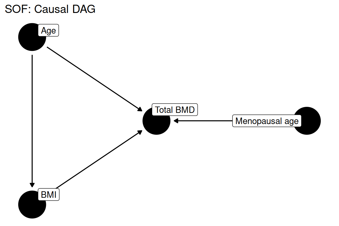
data(sof, package = "rmb")
dat <- haven::zap_labels(sof)
dim(dat)
#> [1] 42950    12
baseline_sof <- subset(dat, visit == 2)
dim(baseline_sof)
#> [1] 8590   12
summary(baseline_sof[c("totbmd", "bmi", "age", "meno_age")])
#>      totbmd            bmi             age           meno_age
#>  Min.   :0.3000   Min.   :15.00   Min.   :67.00   Min.   :14.00
#>  1st Qu.:0.6592   1st Qu.:23.00   1st Qu.:69.00   1st Qu.:45.00
#>  Median :0.7407   Median :26.00   Median :72.00   Median :49.00
#>  Mean   :0.7470   Mean   :26.21   Mean   :73.39   Mean   :48.02
#>  3rd Qu.:0.8268   3rd Qu.:29.00   3rd Qu.:76.00   3rd Qu.:52.00
#>  Max.   :1.4030   Max.   :51.00   Max.   :99.00   Max.   :68.00
#> NAs :377 NAs :783 NAs :35 NAs :1586A linear regression model is fitted at the baseline visit (visit 2) to estimate the cross-sectional association between BMI and total BMD, adjusting for age and menopausal age. Using only baseline visits avoids correlation from repeated measurements (RMB2e Ch. 7).
formula_main <- totbmd ~ bmi + age + meno_age
formula_main
#> totbmd ~ bmi + age + meno_agesummary(baseline_sof[c("totbmd", "bmi", "age", "meno_age")])
#> totbmd bmi age meno_age
#> Min. :0.3000 Min. :15.00 Min. :67.00 Min. :14.00
#> 1st Qu.:0.6592 1st Qu.:23.00 1st Qu.:69.00 1st Qu.:45.00
#> Median :0.7407 Median :26.00 Median :72.00 Median :49.00
#> Mean :0.7470 Mean :26.21 Mean :73.39 Mean :48.02
#> 3rd Qu.:0.8268 3rd Qu.:29.00 3rd Qu.:76.00 3rd Qu.:52.00
#> Max. :1.4030 Max. :51.00 Max. :99.00 Max. :68.00
#> NAs :377 NAs :783 NAs :35 NAs :1586
with(baseline_sof, cor(cbind(totbmd, bmi, age, meno_age), use = "complete.obs"))
#> totbmd bmi age meno_age
#> totbmd 1.00000000 0.45992970 -0.26661905 0.09573091
#> bmi 0.45992970 1.00000000 -0.10440406 0.01762892
#> age -0.26661905 -0.10440406 1.00000000 -0.05340412
#> meno_age 0.09573091 0.01762892 -0.05340412 1.00000000ggplot2::ggplot(baseline_sof, ggplot2::aes(x = bmi, y = totbmd)) +
ggplot2::geom_point(alpha = 0.2, size = 0.8) +
ggplot2::geom_smooth(method = "lm", se = FALSE, color = "#d95f02", linewidth = 1) +
ggplot2::labs(
title = "SOF: Total BMD vs BMI at baseline",
x = expression("BMI (kg/m"^2*")"),
y = "Total BMD (g/cm²)"
) +
ggplot2::theme_minimal()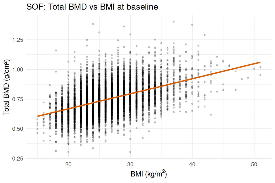
fit <- stats::lm(formula_main, data = baseline_sof)
summary(fit)
#>
#> Call:
#> stats::lm(formula = formula_main, data = baseline_sof)
#>
#> Residuals:
#>      Min       1Q   Median       3Q      Max
#> -0.49349 -0.07361 -0.00646  0.06912  0.62773
#>
#> Coefficients:
#>               Estimate Std. Error t value Pr(>|t|)
#> (Intercept)  0.7402088  0.0253285  29.224  < 2e-16 ***
#> bmi          0.0121491  0.0003008  40.389  < 2e-16 ***
#> age         -0.0053994  0.0002689 -20.082  < 2e-16 ***
#> meno_age     0.0017149  0.0002411   7.112 1.26e-12 ***
#> ---
#> Signif. codes:  0 '***' 0.001 '**' 0.01 '*' 0.05 '.' 0.1 ' ' 1
#>
#> Residual standard error: 0.1092 on 6374 degrees of freedom
#>   (2212 observations deleted due to missingness)
#> Multiple R-squared:  0.2657, Adjusted R-squared:  0.2653
#> F-statistic: 768.7 on 3 and 6374 DF, p-value: < 2.2e-16fit_data <- data.frame(
fitted = stats::fitted(fit),
residuals = stats::residuals(fit),
std_residuals = stats::rstandard(fit)
)
ggplot2::ggplot(fit_data, ggplot2::aes(x = fitted, y = residuals)) +
ggplot2::geom_point(alpha = 0.25, size = 0.5) +
ggplot2::geom_hline(yintercept = 0, linetype = "dashed", color = "red") +
ggplot2::geom_smooth(se = FALSE, color = "blue") +
ggplot2::labs(
title = "Residuals vs Fitted",
x = "Fitted values",
y = "Residuals"
) +
ggplot2::theme_minimal()
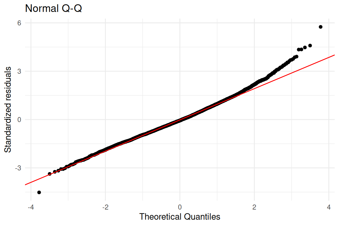
ggplot2::ggplot(fit_data, ggplot2::aes(sample = std_residuals)) +
ggplot2::stat_qq() +
ggplot2::stat_qq_line(color = "red") +
ggplot2::labs(
title = "Normal Q-Q",
x = "Theoretical Quantiles",
y = "Standardized residuals"
) +
ggplot2::theme_minimal()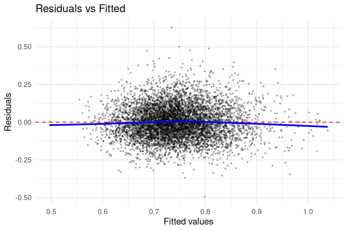
ci <- stats::confint(fit)
coefs <- summary(fit)$coefficients
data.frame(
  term = rownames(coefs),
  estimate = coefs[, "Estimate"],
  conf_low = ci[, 1],
  conf_high = ci[, 2],
  p_value = coefs[, "Pr(>|t|)"]
)
#>                    term     estimate     conf_low    conf_high       p_value
#> (Intercept) (Intercept)  0.740208817  0.690556393  0.789861242 2.640992e-176
#> bmi                 bmi  0.012149083  0.011559408  0.012738759 8.905751e-318
#> age                 age -0.005399411 -0.005926485 -0.004872336  4.993029e-87
#> meno_age meno_age 0.001714878 0.001242226 0.002187530 1.264228e-12Higher BMI is positively associated with total BMD at baseline after adjustment for age and menopausal age in SOF women, consistent with the mechanical loading and estrogenic pathways described above (RMB2e Ch. 7). Age is negatively associated with BMD, reflecting postmenopausal bone loss. Menopausal age contributes independently, as women who underwent menopause later experienced fewer years of estrogen deficiency. This cross-sectional analysis uses only Visit 2 data (the earliest available visit in the SOF dataset) to avoid the need for mixed-model methods introduced for the longitudinal SOF analyses elsewhere in RMB2e.