Code
data(rmb_datasets, package = "rmb")
rmb_datasets$study_design[rmb_datasets$object == "fecfat"]
#> [1] "Repeated-measures study comparing pancreatic enzyme regimens using fecal fat outcomes."This article analyzes the fecal fat crossover experiment, testing whether different pill types affect mean fecal fat output while accounting for within-subject correlation (RMB2e Chapter 7).
Fecal fat excretion is a sensitive marker of intestinal fat malabsorption and has been used to evaluate the efficacy of pancreatic enzyme replacement and other GI interventions. This small crossover experiment assigned subjects to different pill formulations sequentially, measuring daily fecal fat (g/day) under each condition. The repeated-measures design means that fecal fat values from the same subject are correlated; failure to account for this within-subject variability would inflate standard errors or deflate them inappropriately (RMB2e Ch. 7).
data(rmb_datasets, package = "rmb")
rmb_datasets$study_design[rmb_datasets$object == "fecfat"]
#> [1] "Repeated-measures study comparing pancreatic enzyme regimens using fecal fat outcomes."Do different pill types differ in mean fecal fat output, accounting for within-subject correlation?
set.seed(42)
dag <- ggdag::dagify(
  fecfat ~ pill + subject,
  labels = c(
    fecfat = "Fecal fat (g/day)",
    pill = "Pill type",
    subject = "Subject/patient"
  ),
  exposure = "pill",
  outcome = "fecfat"
)
ggdag::ggdag(dag, use_labels = "label", text = FALSE) +
  ggdag::theme_dag_blank() +
  ggplot2::labs(title = "Fecal fat: Causal DAG")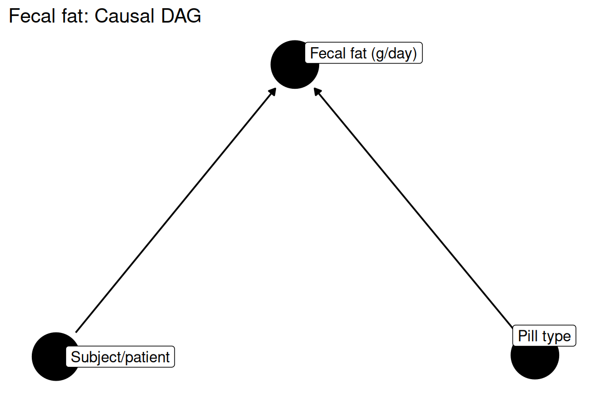
data(fecfat, package = "rmb")
dat <- fecfat
dim(dat)
#> [1] 24  3
summary(haven::zap_labels(dat[c("fecfat", "pilltype", "subject")]))
#>      fecfat          pilltype       subject
#>  Min.   : 3.400   Min.   :1.00   Min.   :1.0
#>  1st Qu.: 8.875   1st Qu.:1.75   1st Qu.:2.0
#>  Median :22.550   Median :2.50   Median :3.5
#>  Mean   :25.775   Mean   :2.50   Mean   :3.5
#>  3rd Qu.:36.500   3rd Qu.:3.25   3rd Qu.:5.0
#> Max. :71.300 Max. :4.00 Max. :6.0A linear model with subject included as a blocking factor is used to remove between-subject variability and isolate the pill type effect, equivalent to a one-way ANOVA within subjects (RMB2e Ch. 7).
with(dat, tapply(fecfat, pilltype, summary))
#> $`1`
#>    Min. 1st Qu.  Median    Mean 3rd Qu.    Max.
#>    9.40   22.57   38.75   38.08   49.53   71.30
#>
#> $`2`
#>    Min. 1st Qu.  Median    Mean 3rd Qu.    Max.
#>   4.600   5.575  14.150  16.533  22.725  38.000
#>
#> $`3`
#>    Min. 1st Qu.  Median    Mean 3rd Qu.    Max.
#>    3.40    6.40   17.45   17.42   24.98   36.00
#>
#> $`4`
#>    Min. 1st Qu.  Median    Mean 3rd Qu.    Max.
#>    5.80   14.80   23.70   31.07   45.80   68.20
with(dat, tapply(fecfat, subject, mean))
#>      1      2      3      4      5      6
#> 16.900 25.625 14.475 6.100 47.100 44.450ggplot2::ggplot(dat, ggplot2::aes(x = pilltype, y = fecfat)) +
ggplot2::geom_boxplot(fill = "#d95f02") +
ggplot2::labs(
title = "Fecal fat by pill type",
x = "Pill type",
y = "Fecal fat (g/day)"
) +
ggplot2::theme_minimal()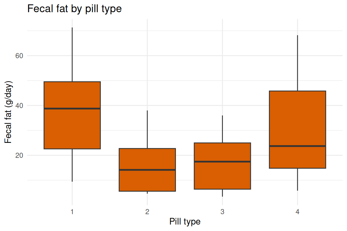
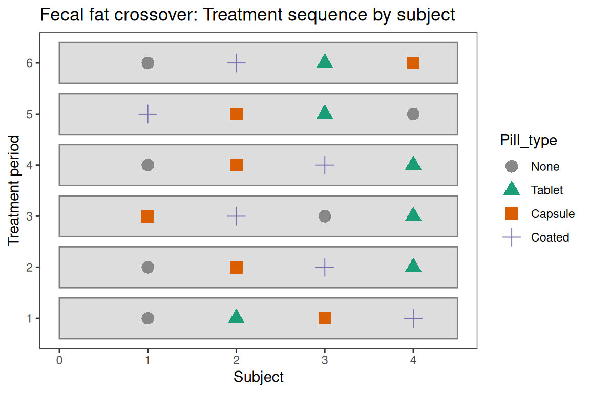
The swimmer plot below shows the treatment sequence for each of the 6 subjects, with colored symbols indicating which pill type was assigned in each of the four periods.
dat_swim <- as.data.frame(dat)
dat_swim$pilltype_int <- as.integer(unclass(dat_swim$pilltype))
dat_swim$Pill_type <- factor(
  dat_swim$pilltype_int,
  levels = 1:4,
  labels = c("None", "Tablet", "Capsule", "Coated")
)
dat_swim$subject_int <- as.integer(dat_swim$subject)
dat_swim$period <- as.integer(
  ave(seq_len(nrow(dat_swim)), dat_swim$subject_int, FUN = seq_along)
)

# One row per subject for the background bar
dat_sum <- data.frame(
  subject_int = sort(unique(dat_swim$subject_int)),
  end = 4.5
)

swimplot::swimmer_plot(
  df = dat_sum, id = "subject_int", end = "end",
  increasing = FALSE, col = "grey50", alpha = 0.2, width = 0.8
) +
  swimplot::swimmer_points(
    df = dat_swim, id = "subject_int", time = "period",
    name_col = "Pill_type", name_shape = "Pill_type", size = 4
  ) +
  ggplot2::scale_colour_manual(
    values = c("#888888", "#1b9e77", "#d95f02", "#7570b3")
  ) +
  ggplot2::labs(
    x = "Treatment period",
    y = "Subject",
    title = "Fecal fat crossover: Treatment sequence by subject"
  )
fit <- stats::lm(formula_main, data = dat)
summary(fit)
#>
#> Call:
#> stats::lm(formula = formula_main, data = dat)
#>
#> Residuals:
#>      Min       1Q   Median       3Q      Max
#> -14.5583  -5.5667  -0.1625   5.7208  15.8083
#>
#> Coefficients:
#>             Estimate Std. Error t value Pr(>|t|)
#> (Intercept)   29.208      6.334   4.611 0.000339 ***
#> pilltype2    -21.550      5.972  -3.608 0.002581 **
#> pilltype3    -20.667      5.972  -3.461 0.003496 **
#> pilltype4     -7.017      5.972  -1.175 0.258348
#> subject2       8.725      7.314   1.193 0.251451
#> subject3      -2.425      7.314  -0.332 0.744823
#> subject4     -10.800      7.314  -1.477 0.160480
#> subject5      30.200      7.314   4.129 0.000892 ***
#> subject6      27.550      7.314   3.767 0.001867 **
#> ---
#> Signif. codes:  0 '***' 0.001 '**' 0.01 '*' 0.05 '.' 0.1 ' ' 1
#>
#> Residual standard error: 10.34 on 15 degrees of freedom
#> Multiple R-squared:  0.8256, Adjusted R-squared:  0.7326
#> F-statistic: 8.875 on 8 and 15 DF, p-value: 0.0001758fit_data <- data.frame(
fitted = stats::fitted(fit),
residuals = stats::residuals(fit),
std_residuals = stats::rstandard(fit)
)
ggplot2::ggplot(fit_data, ggplot2::aes(x = fitted, y = residuals)) +
ggplot2::geom_point() +
ggplot2::geom_hline(yintercept = 0, linetype = "dashed", color = "red") +
ggplot2::geom_smooth(se = FALSE, color = "blue") +
ggplot2::labs(
title = "Residuals vs Fitted",
x = "Fitted values",
y = "Residuals"
) +
ggplot2::theme_minimal()
ggplot2::ggplot(fit_data, ggplot2::aes(sample = std_residuals)) +
ggplot2::stat_qq() +
ggplot2::stat_qq_line(color = "red") +
ggplot2::labs(
title = "Normal Q-Q",
x = "Theoretical Quantiles",
y = "Standardized residuals"
) +
ggplot2::theme_minimal()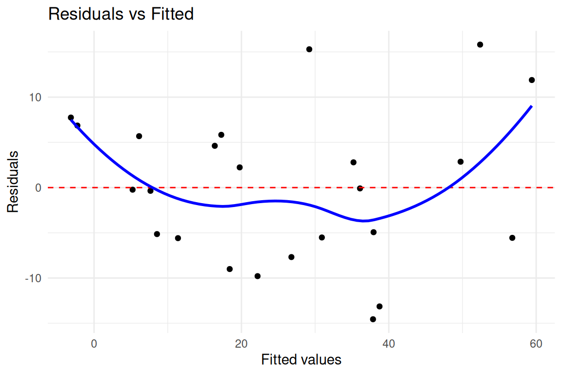
ci <- stats::confint(fit)
coefs <- summary(fit)$coefficients
pill_rows <- grep("^pilltype", rownames(coefs))
data.frame(
  term = rownames(coefs)[pill_rows],
  estimate = coefs[pill_rows, "Estimate"],
  conf_low = ci[pill_rows, 1],
  conf_high = ci[pill_rows, 2],
  p_value = coefs[pill_rows, "Pr(>|t|)"]
)
#>                term   estimate  conf_low conf_high     p_value
#> pilltype2 pilltype2 -21.550001 -34.27929 -8.820714 0.002580662
#> pilltype3 pilltype3 -20.666667 -33.39595 -7.937381 0.003495554
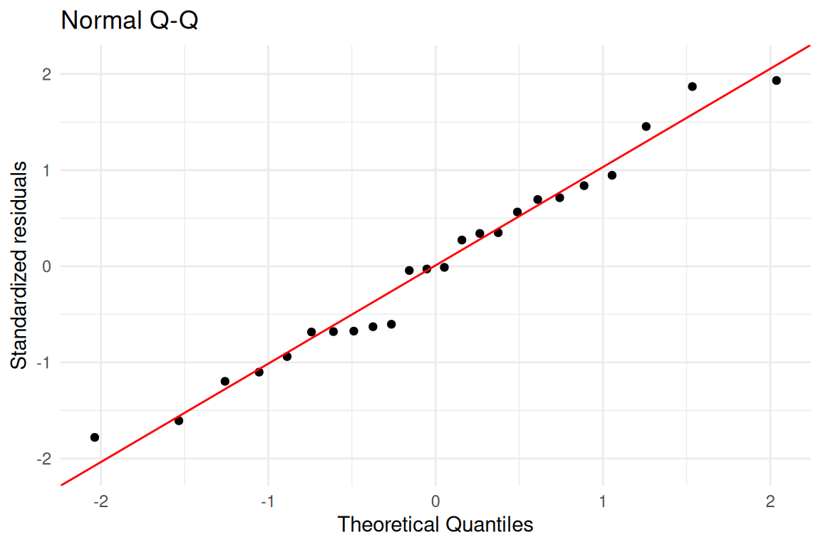
#> pilltype4 pilltype4 -7.016668 -19.74595 5.712618 0.258348026After blocking on subject identity to remove between-subject variability, differences in mean fecal fat across pill types reflect the within-subject treatment effect of each formulation (RMB2e Ch. 7). This design is particularly powerful because it eliminates the dominant source of variation (subject-to-subject differences in baseline fat excretion), allowing a relatively small crossover study to detect meaningful differences. The residual plots confirm the adequacy of the linear model for inference.