Leukemia data

This article reproduces the leukemia remission survival analysis from Freireich et al. (1963), comparing 6-mercaptopurine and placebo using Kaplan-Meier curves and a log-rank test as introduced in RMB2e Chapter 3.

1 Introduction

Acute lymphoblastic leukemia (ALL) in adults historically carried a poor prognosis, with complete remission rates that were short-lived without maintenance therapy. Freireich and colleagues (1963) conducted a landmark randomized crossover trial comparing 6-mercaptopurine (6-MP) to placebo in patients achieving complete remission, measuring time until relapse. This small dataset (42 patients, 21 per group) is a canonical teaching example for survival analysis because it clearly illustrates the Kaplan-Meier estimator and the log-rank test (RMB2e Ch. 3).

Code

data(rmb_datasets, package = "rmb")
rmb_datasets$study_design[rmb_datasets$object == "leuk"]
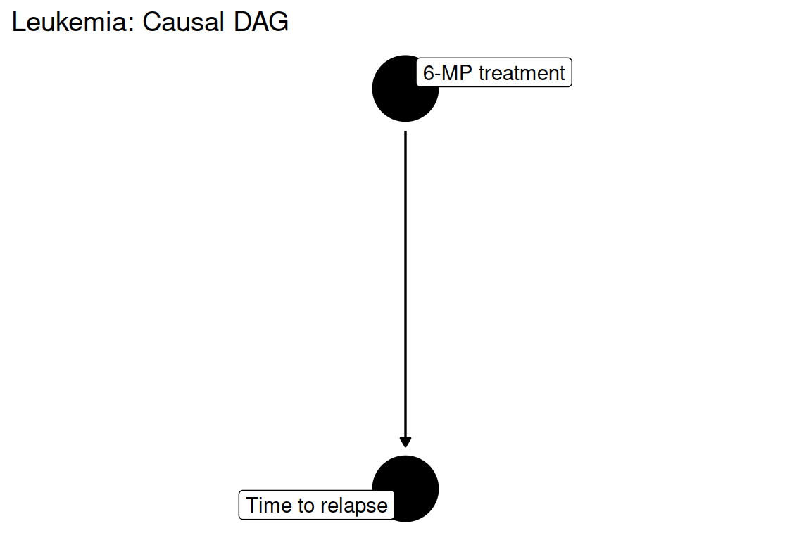
#> [1] "Randomized acute lymphoblastic leukemia remission trial comparing 6-MP versus placebo."

Does 6-MP treatment prolong leukemia remission compared to placebo?

1.1 Causal assumptions

Code

set.seed(42)
dag <- ggdag::dagify(
  time_relapse ~ rx,
  labels = c(time_relapse = "Time to relapse", rx = "6-MP treatment"),
  exposure = "rx",
  outcome = "time_relapse"
)
ggdag::ggdag(dag, use_labels = "label", text = FALSE) +
  ggdag::theme_dag_blank() +
  ggplot2::labs(title = "Leukemia: Causal DAG")

Figure 1: Directed acyclic graph for the leukemia remission treatment comparison.

2 Methods

2.1 Study sample

Code

data(leuk, package = "rmb")
dat <- leuk
dim(dat)
#> [1] 42  3
summary(haven::zap_labels(dat[c("time", "cens", "group")]))
#>       time            cens            group    
#>  Min.   : 1.00   Min.   :0.0000   Min.   :1.0  
#>  1st Qu.: 6.00   1st Qu.:0.0000   1st Qu.:1.0  
#>  Median :10.50   Median :1.0000   Median :1.5  
#>  Mean   :12.88   Mean   :0.7143   Mean   :1.5  
#>  3rd Qu.:18.50   3rd Qu.:1.0000   3rd Qu.:2.0  
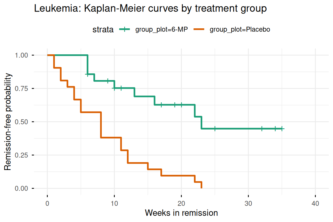
#>  Max.   :35.00   Max.   :1.0000   Max.   :2.0

2.2 Statistical analysis

Kaplan-Meier curves are estimated by treatment group, and the log-rank test is used to assess the null hypothesis of equal survival functions. The 6-MP vs placebo comparison was randomized, so no covariate adjustment is needed for valid inference (RMB2e Ch. 3).

Code

surv_obj <- survival::Surv(dat$time, dat$cens)
km_formula <- surv_obj ~ group
km_formula
#> surv_obj ~ group

3 Results

3.1 Descriptive statistics

Code

with(dat, tapply(time, group, summary))
#> $`1`
#>    Min. 1st Qu.  Median    Mean 3rd Qu.    Max. 
#>     6.0     9.0    16.0    17.1    23.0    35.0 
#> 
#> $`2`
#>    Min. 1st Qu.  Median    Mean 3rd Qu.    Max. 
#>   1.000   4.000   8.000   8.667  12.000  23.000
with(dat, tapply(cens, group, mean))
#>         1         2 
#> 0.4285714 1.0000000

Code

treatment_group_labels <- c(`1` = "6-MP", `2` = "Placebo")
treatment_palette <- c("6-MP" = "#1b9e77", "Placebo" = "#d95f02")
dat$group_plot <- factor(
  dat$group,
  levels = c(1, 2),
  labels = treatment_group_labels
)
km_fit <- survival::survfit(survival::Surv(time, cens) ~ group_plot, data = dat)

survminer::ggsurvplot(
  km_fit,
  data = dat,
  title = "Leukemia: Kaplan-Meier curves by treatment group",
  xlab = "Weeks in remission",
  ylab = "Remission-free probability",
  legend.title = NULL,
  ggtheme = ggplot2::theme_minimal(),
  palette = unname(treatment_palette),
  conf.int = FALSE,
  censor = TRUE
)

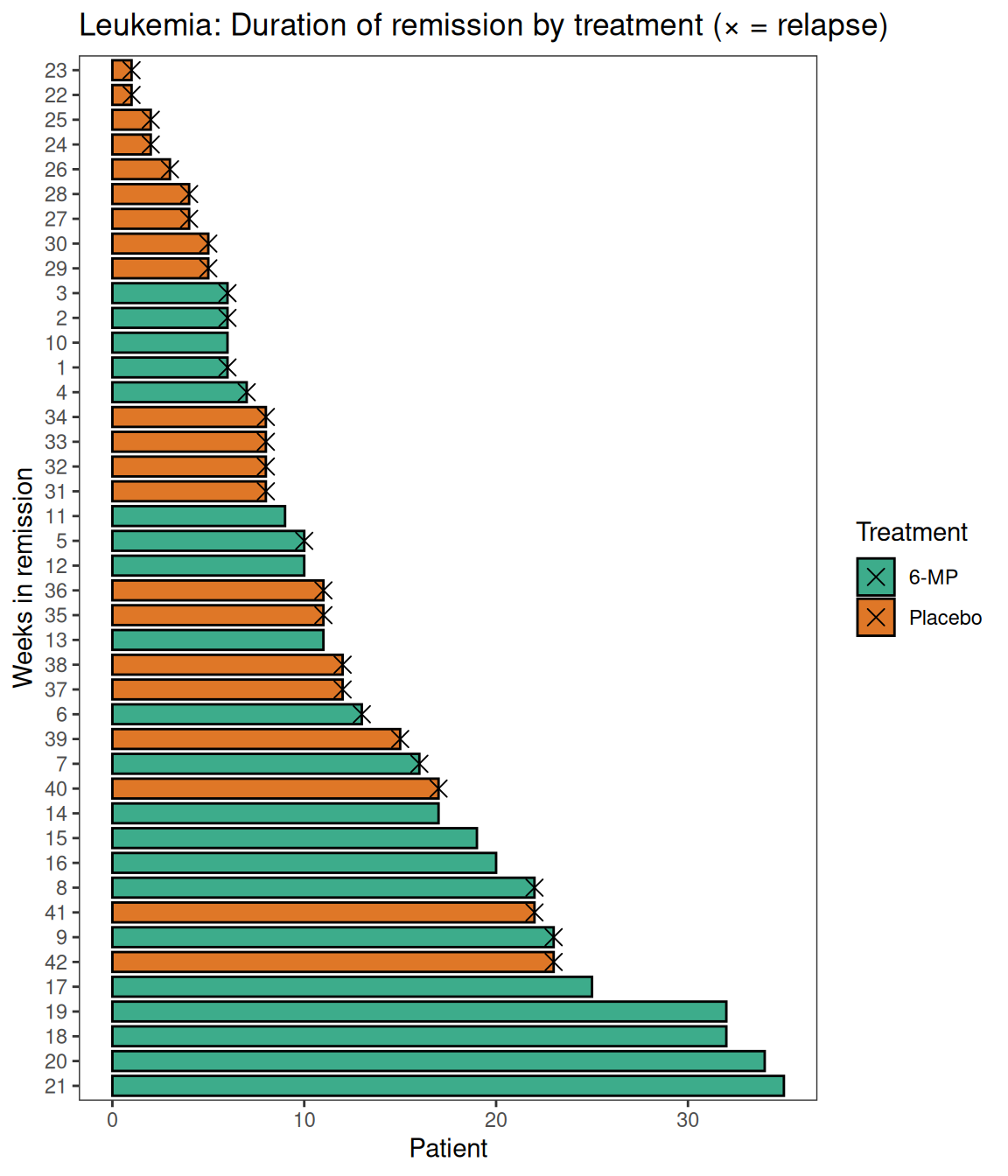
Figure 2: Kaplan-Meier remission curves comparing 6-MP and placebo groups.

All 42 participants can be shown in a swimmer plot, displaying each individual’s time in remission with relapses marked by an ×.

Code

dat_swim <- as.data.frame(dat)
dat_swim$id <- seq_len(nrow(dat_swim))
dat_swim$time <- as.numeric(dat_swim$time)
dat_swim$group_int <- as.integer(unclass(dat_swim$group))
dat_swim$Treatment <- factor(
  dat_swim$group_int,
  levels = c(1, 2),
  labels = treatment_group_labels
)
dat_relapse <- dat_swim[dat_swim$cens == 1, ]

swimplot::swimmer_plot(
  df = dat_swim, id = "id", end = "time",
  name_fill = "Treatment", increasing = FALSE,
  col = "black", alpha = 0.85, width = 0.8
) +
  swimplot::swimmer_points(
    df = dat_relapse, id = "id", time = "time",
    shape = 4, size = 3, col = "black"
  ) +
  ggplot2::scale_fill_manual(values = treatment_palette) +
  ggplot2::labs(
    x = "Weeks in remission",
    y = "Patient",
    title = "Leukemia: Duration of remission by treatment (× = relapse)"
  )

Figure 3: Swimmer plot of remission duration with relapse markers for all patients.

3.2 Model estimates

Code

km_fit
#> Call: survfit(formula = survival::Surv(time, cens) ~ group_plot, data = dat)
#> 
#>                     n events median 0.95LCL 0.95UCL
#> group_plot=6-MP    21      9     23      16      NA
#> group_plot=Placebo 21     21      8       4      12
summary(km_fit)
#> Call: survfit(formula = survival::Surv(time, cens) ~ group_plot, data = dat)
#> 
#>                 group_plot=6-MP 
#>  time n.risk n.event survival std.err lower 95% CI upper 95% CI
#>     6     21       3    0.857  0.0764        0.720        1.000
#>     7     17       1    0.807  0.0869        0.653        0.996
#>    10     15       1    0.753  0.0963        0.586        0.968
#>    13     12       1    0.690  0.1068        0.510        0.935
#>    16     11       1    0.627  0.1141        0.439        0.896
#>    22      7       1    0.538  0.1282        0.337        0.858
#>    23      6       1    0.448  0.1346        0.249        0.807
#> 
#>                 group_plot=Placebo 
#>  time n.risk n.event survival std.err lower 95% CI upper 95% CI
#>     1     21       2   0.9048  0.0641      0.78754        1.000
#>     2     19       2   0.8095  0.0857      0.65785        0.996
#>     3     17       1   0.7619  0.0929      0.59988        0.968
#>     4     16       2   0.6667  0.1029      0.49268        0.902
#>     5     14       2   0.5714  0.1080      0.39455        0.828
#>     8     12       4   0.3810  0.1060      0.22085        0.657
#>    11      8       2   0.2857  0.0986      0.14529        0.562
#>    12      6       2   0.1905  0.0857      0.07887        0.460
#>    15      4       1   0.1429  0.0764      0.05011        0.407
#>    17      3       1   0.0952  0.0641      0.02549        0.356
#>    22      2       1   0.0476  0.0465      0.00703        0.322
#>    23      1       1   0.0000     NaN           NA           NA

3.3 Model diagnostics

Code

logrank_test <- survival::survdiff(survival::Surv(time, cens) ~ group, data = dat)
logrank_test
#> Call:
#> survival::survdiff(formula = survival::Surv(time, cens) ~ group, 
#>     data = dat)
#> 
#>          N Observed Expected (O-E)^2/E (O-E)^2/V
#> group=1 21        9     19.3      5.46      16.8
#> group=2 21       21     10.7      9.77      16.8
#> 
#>  Chisq= 16.8  on 1 degrees of freedom, p= 4e-05

3.4 Inference

Code

chi2 <- logrank_test$chisq
df <- length(logrank_test$n) - 1
p_val <- 1 - stats::pchisq(chi2, df = df)
knitr::kable(data.frame(
  test = "log-rank",
  chi_squared = round(chi2, 3),
  df = df,
  p_value = signif(p_val, 3)
), digits = 3)

Table 1: Log-rank test results comparing remission curves across treatment groups.

test	chi_squared	df	p_value
log-rank	16.793	1	0

4 Discussion

The Kaplan-Meier curves show a marked separation between the 6-MP and placebo groups throughout the follow-up period, and the log-rank test provides strong evidence against equal survival functions (RMB2e Ch. 3). Median remission duration is substantially longer in the 6-MP group, mirroring the original report by Freireich et al. (1963). This analysis serves as a foundational example of how nonparametric survival methods can compare treatment groups without distributional assumptions, motivating the Cox regression approach introduced in later chapters.

5 Source

Freireich EJ et al. (1963). The effect of 6-mercaptopurine on the duration of steroid-induced remissions in acute leukemia. Blood, 21, 699–716.
UCSF Regression Methods companion data: https://regression.ucsf.edu/sites/g/files/tkssra16191/files/wysiwyg/home/data/leuk.dta
Book: Vittinghoff E, Glidden DV, Shiboski SC, McCulloch CE (2012). Regression Methods in Biostatistics (2nd edition).