Code
data(rmb_datasets, package = "rmb")
rmb_datasets$study_design[rmb_datasets$object == "gababies"]
#> [1] "Clustered repeated-birth sample from Georgia mothers used for birthweight analyses."This article examines whether maternal age and interpregnancy interval are associated with infant birthweight in clustered Georgia birth records, illustrating the challenges of correlated outcomes in RMB2e Chapter 7.
Birthweight is a key neonatal health indicator strongly predicted by gestational age, maternal weight, and parity-related factors. When multiple births are recorded per mother, infant outcomes within the same mother are correlated— violating the independence assumption of ordinary linear regression. The Georgia births dataset (gababies) provides a clustered sample of 1,000 birth records from mothers with multiple deliveries, enabling study of between- and within-mother predictors of birthweight (RMB2e Ch. 7).
data(rmb_datasets, package = "rmb")
rmb_datasets$study_design[rmb_datasets$object == "gababies"]
#> [1] "Clustered repeated-birth sample from Georgia mothers used for birthweight analyses."Are maternal age and interpregnancy interval associated with infant birthweight, after accounting for clustering of births within mothers?
set.seed(42)
dag <- ggdag::dagify(
  bw ~ momage + interval + initwt,
  interval ~ momage,
  labels = c(
    bw = "Birthweight",
    momage = "Maternal age",
    interval = "Interpregnancy interval",
    initwt = "Initial maternal weight"
  ),
  exposure = "interval",
  outcome = "bw"
)
ggdag::ggdag(dag, use_labels = "label", text = FALSE) +
  ggdag::theme_dag_blank() +
  ggplot2::labs(title = "GABABabies: Causal DAG")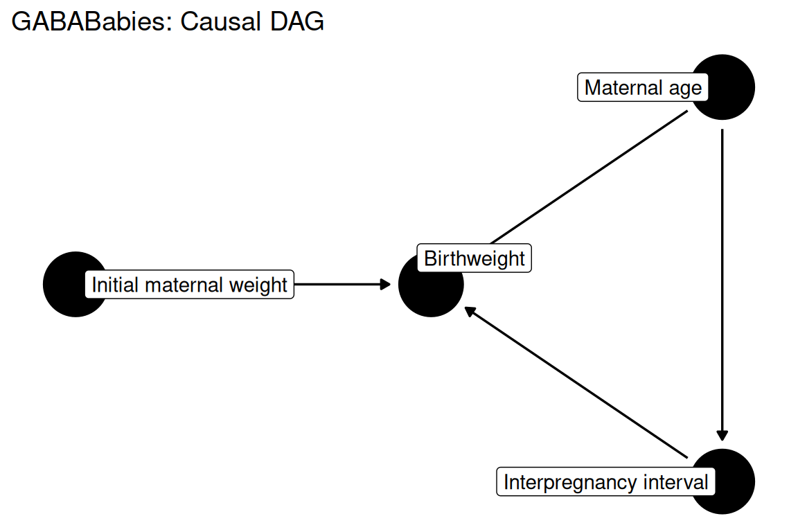
data(gababies, package = "rmb")
dat <- gababies
dim(dat)
#> [1] 1000   11
summary(haven::zap_labels(dat[c("bweight", "cinitage", "timesnc", "momage", "delwght")]))
#>     bweight        cinitage         timesnc           momage
#>  Min.   : 340   Min.   :-5.545   Min.   :-8.000   Min.   :12.00
#>  1st Qu.:2835   1st Qu.:-2.545   1st Qu.: 1.000   1st Qu.:18.00
#>  Median :3175   Median :-0.545   Median : 4.000   Median :21.00
#>  Mean   :3135   Mean   : 0.000   Mean   : 4.088   Mean   :21.63
#>  3rd Qu.:3487   3rd Qu.: 0.455   3rd Qu.: 6.000   3rd Qu.:24.00
#>  Max.   :5018   Max.   :14.455   Max.   :81.000   Max.   :99.00
#>     delwght
#>  Min.   :-1551.0
#>  1st Qu.: -190.0
#>  Median :  164.0
#>  Mean   :  191.6
#>  3rd Qu.:  482.0
#> Max. : 2700.0A linear regression of birthweight on centered maternal age at first birth (cinitage), interpregnancy interval (timesnc), and current maternal age is fitted, ignoring clustering for a baseline OLS estimate; the discussion notes the need for mixed-effects models to account for within-mother correlation (RMB2e Ch. 7).
formula_main <- bweight ~ cinitage + timesnc + momage
formula_main
#> bweight ~ cinitage + timesnc + momagewith(dat, tapply(bweight, birthord, summary))
#> $`1`
#> Min. 1st Qu. Median Mean 3rd Qu. Max.
#> 815 2818 3051 3017 3349 4508
#>
#> $`2`
#> Min. 1st Qu. Median Mean 3rd Qu. Max.
#> 1021 2835 3154 3111 3430 4678
#>
#> $`3`
#> Min. 1st Qu. Median Mean 3rd Qu. Max.
#> 340 2828 3202 3147 3521 4960
#>
#> $`4`
#> Min. 1st Qu. Median Mean 3rd Qu. Max.
#> 910 2892 3246 3194 3525 4780
#>
#> $`5`
#> Min. 1st Qu. Median Mean 3rd Qu. Max.
#> 1210 2854 3218 3208 3548 5018
with(dat, c(n_mothers = length(unique(momid)), n_births = nrow(dat)))
#> n_mothers n_births
#> 200 1000
summary(haven::zap_labels(dat[c("bweight", "cinitage", "timesnc")]))
#> bweight cinitage timesnc
#> Min. : 340 Min. :-5.545 Min. :-8.000
#> 1st Qu.:2835 1st Qu.:-2.545 1st Qu.: 1.000
#> Median :3175 Median :-0.545 Median : 4.000
#> Mean :3135 Mean : 0.000 Mean : 4.088
#> 3rd Qu.:3487 3rd Qu.: 0.455 3rd Qu.: 6.000
#> Max. :5018 Max. :14.455 Max. :81.000ggplot2::ggplot(dat, ggplot2::aes(x = factor(birthord), y = bweight)) +
ggplot2::geom_boxplot(fill = "grey85") +
ggplot2::labs(
title = "Georgia births: Birthweight by birth order",
x = "Birth order",
y = "Birthweight (grams)"
) +
ggplot2::theme_minimal()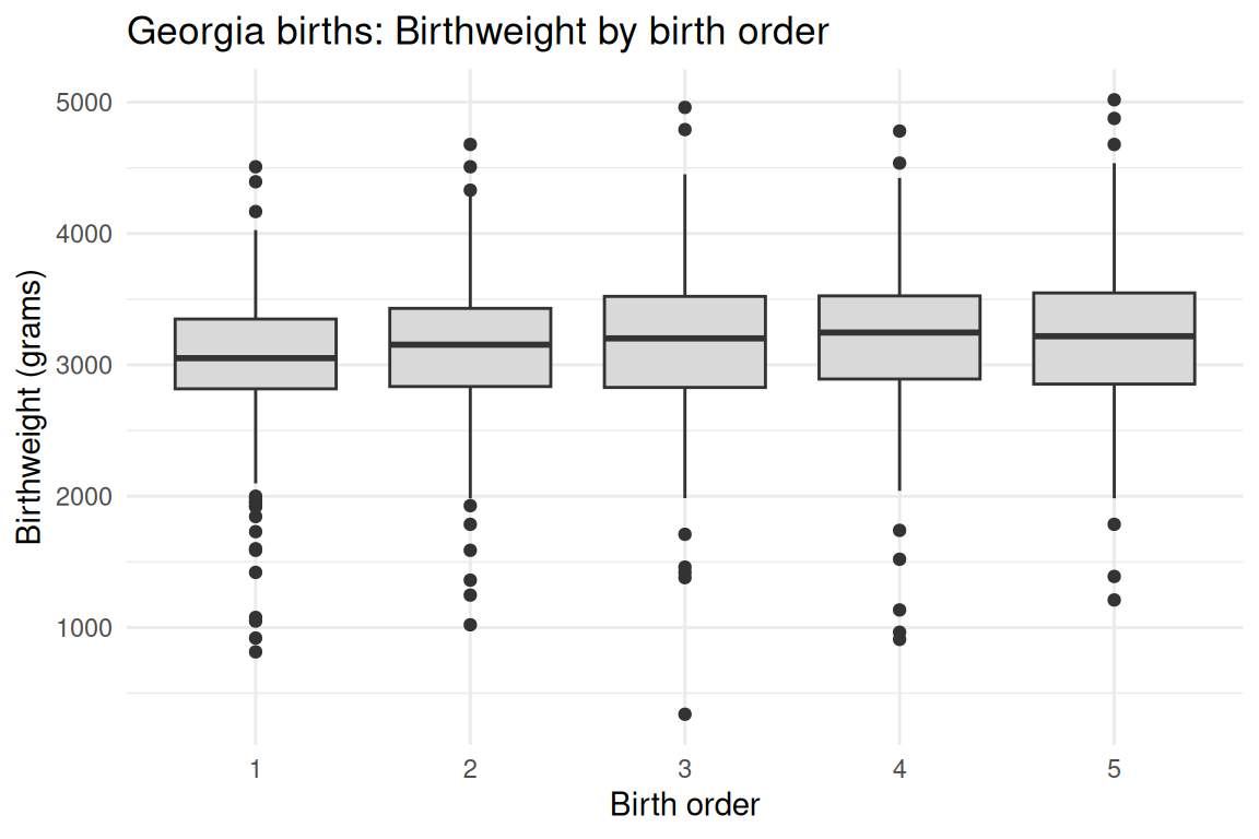
fit <- stats::lm(formula_main, data = dat)
summary(fit)
#>
#> Call:
#> stats::lm(formula = formula_main, data = dat)
#>
#> Residuals:
#>      Min       1Q   Median       3Q      Max
#> -2990.00  -301.41    31.64   332.68  1721.94
#>
#> Coefficients: (1 not defined because of singularities)
#>             Estimate Std. Error t value Pr(>|t|)
#> (Intercept) 3079.486     23.716 129.846  < 2e-16 ***
#> cinitage      26.082      5.608   4.650 3.76e-06 ***
#> timesnc       13.693      3.766   3.636 0.000291 ***
#> momage            NA         NA      NA       NA
#> ---
#> Signif. codes:  0 '***' 0.001 '**' 0.01 '*' 0.05 '.' 0.1 ' ' 1
#>
#> Residual standard error: 570.5 on 997 degrees of freedom
#> Multiple R-squared:  0.03482,    Adjusted R-squared:  0.03288
#> F-statistic: 17.98 on 2 and 997 DF, p-value: 2.129e-08fit_data <- data.frame(
fitted = stats::fitted(fit),
residuals = stats::residuals(fit),
std_residuals = stats::rstandard(fit)
)
ggplot2::ggplot(fit_data, ggplot2::aes(x = fitted, y = residuals)) +
ggplot2::geom_point() +
ggplot2::geom_hline(yintercept = 0, linetype = "dashed", color = "red") +
ggplot2::geom_smooth(se = FALSE, color = "blue") +
ggplot2::labs(
title = "Residuals vs Fitted",
x = "Fitted values",
y = "Residuals"
) +
ggplot2::theme_minimal()
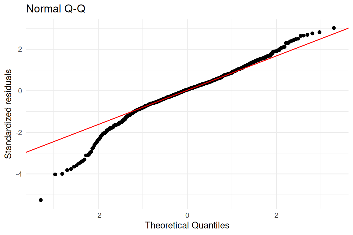
ggplot2::ggplot(fit_data, ggplot2::aes(sample = std_residuals)) +
ggplot2::stat_qq() +
ggplot2::stat_qq_line(color = "red") +
ggplot2::labs(
title = "Normal Q-Q",
x = "Theoretical Quantiles",
y = "Standardized residuals"
) +
ggplot2::theme_minimal()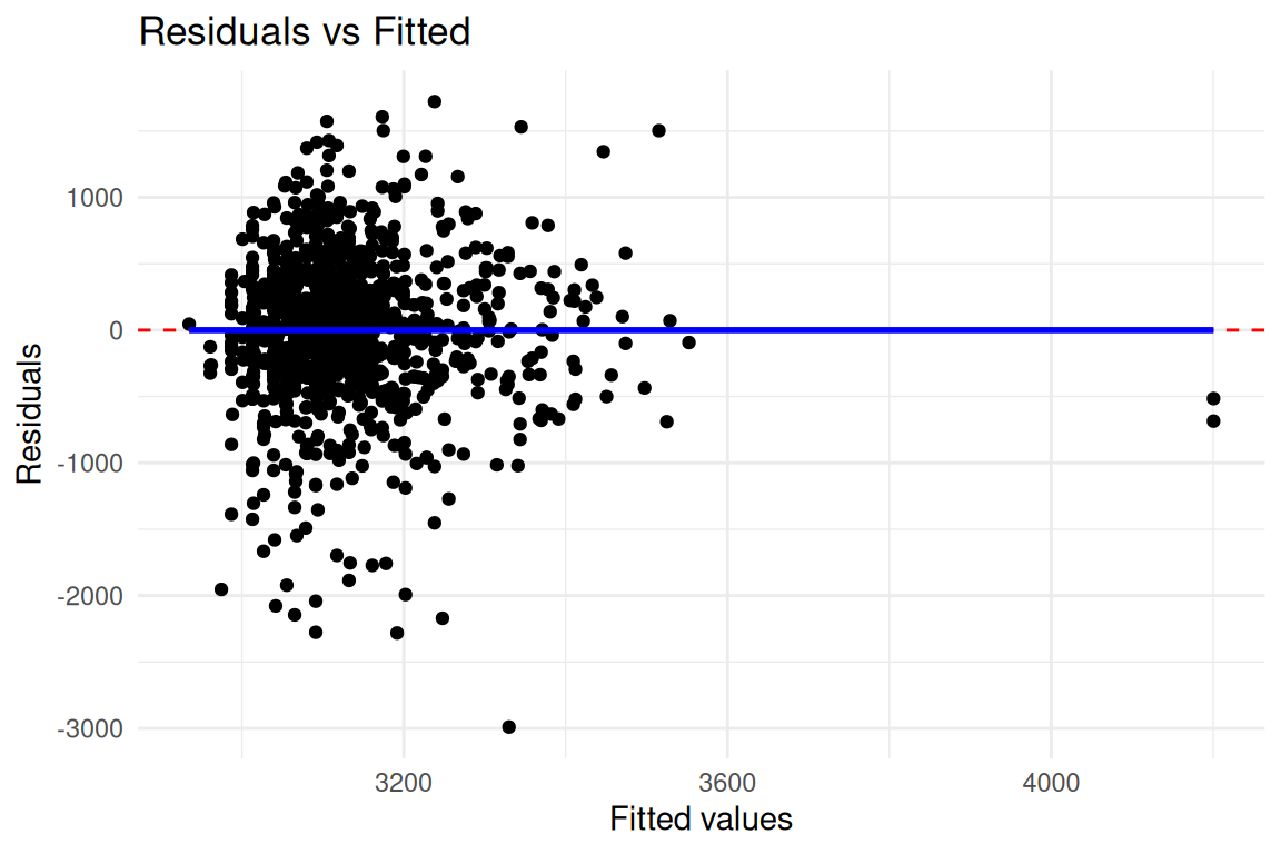
ci <- stats::confint(fit)
coefs <- summary(fit)$coefficients
ci_sub <- ci[rownames(coefs), , drop = FALSE]
data.frame(
  term = rownames(coefs),
  estimate = coefs[, "Estimate"],
  conf_low = ci_sub[, 1],
  conf_high = ci_sub[, 2],
  p_value = coefs[, "Pr(>|t|)"]
)
#>                    term   estimate    conf_low  conf_high      p_value
#> (Intercept) (Intercept) 3079.48641 3032.946433 3126.02639 0.000000e+00
#> cinitage       cinitage   26.08179   15.076064   37.08752 3.757601e-06
#> timesnc timesnc 13.69315 6.303301 21.08299 2.908827e-04The OLS estimates show the direction of associations between maternal characteristics and birthweight, but standard errors underestimate uncertainty because births within the same mother are correlated (RMB2e Ch. 7). Proper inference requires a mixed-effects model with a random intercept for mother, which would partition the total variance into within-mother and between-mother components. The centered age at first birth (cinitage) isolates the between-mother age effect, while timesnc captures the interpregnancy interval’s influence on fetal growth.