Code
data(rmb_datasets, package = "rmb")
rmb_datasets$study_design[rmb_datasets$object == "fit"]
#> [1] "Randomized Fracture Intervention Trial of alendronate in postmenopausal women."This article fits a logistic regression model to the Fracture Intervention Trial (FIT) dataset, evaluating whether alendronate reduces new vertebral fracture incidence in postmenopausal women (RMB2e Chapter 6).
Postmenopausal osteoporosis is characterized by rapid bone loss driven by estrogen deficiency, leading to increased fracture risk. The Fracture Intervention Trial (FIT) was a large randomized placebo-controlled trial of the bisphosphonate alendronate in postmenopausal women with low femoral neck BMD (Black et al. 1996). New vertebral fractures were identified from serial lateral spine radiographs and serve as the primary binary outcome in this analysis. A history of prior vertebral fracture and low baseline BMD are strong confounders and are included as adjusters (RMB2e Ch. 6).
data(rmb_datasets, package = "rmb")
rmb_datasets$study_design[rmb_datasets$object == "fit"]
#> [1] "Randomized Fracture Intervention Trial of alendronate in postmenopausal women."Does alendronate treatment reduce the incidence of new vertebral fractures compared to placebo in postmenopausal women with low BMD?
set.seed(42)
dag <- ggdag::dagify(
  vfx ~ treat + age + fracbase + bmdbase,
  treat ~ bmdbase,
  labels = c(
    vfx = "New vertebral fx",
    treat = "Alendronate",
    age = "Age",
    fracbase = "Prior fx",
    bmdbase = "Baseline BMD"
  ),
  exposure = "treat",
  outcome = "vfx"
)
ggdag::ggdag(dag, use_labels = "label", text = FALSE) +
  ggdag::theme_dag_blank() +
  ggplot2::labs(title = "FIT: Causal DAG")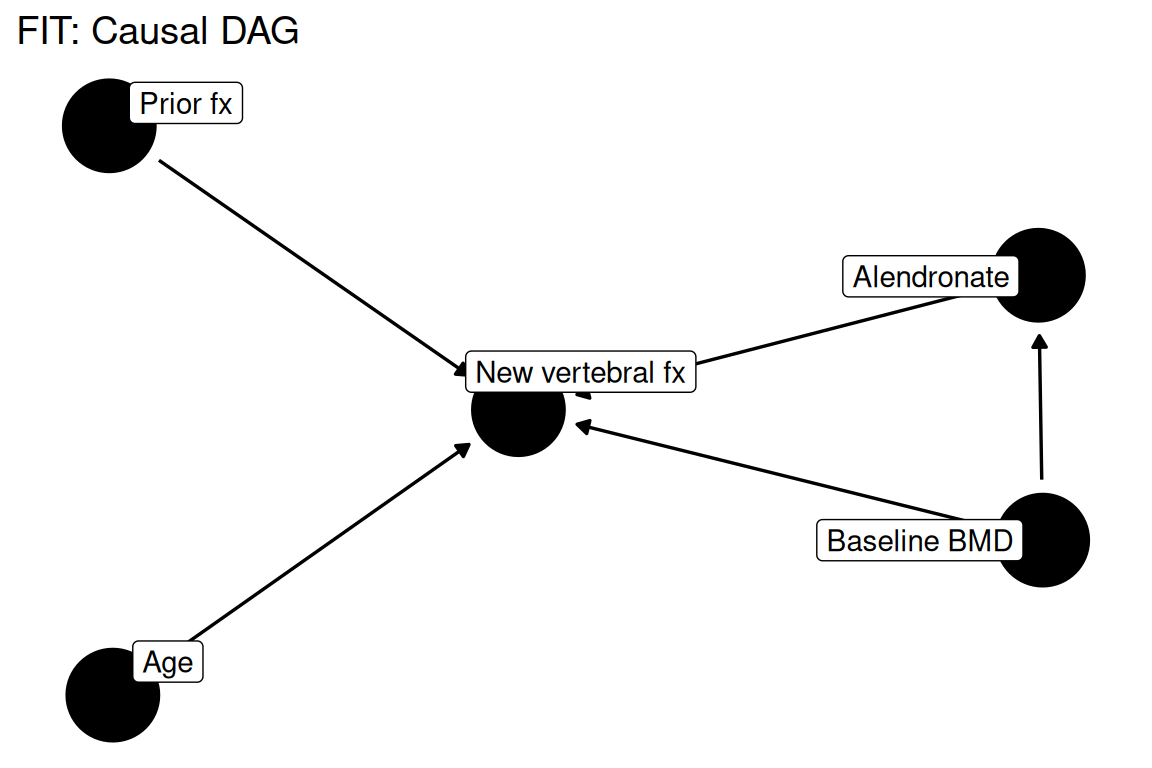
data(fit, package = "rmb")
dat <- fit
dim(dat)
#> [1] 5324    9
summary(haven::zap_labels(dat[c("treat", "age", "frac_base", "bmd_base", "newvfx", "fitpy")]))
#>      treat             age          frac_base         bmd_base
#>  Min.   :0.0000   Min.   :55.05   Min.   :0.0000   Min.   : 5.432
#>  1st Qu.:0.0000   1st Qu.:64.00   1st Qu.:0.0000   1st Qu.: 8.509
#>  Median :0.0000   Median :68.33   Median :0.0000   Median : 9.278
#>  Mean   :0.4987   Mean   :68.27   Mean   :0.3116   Mean   : 9.183
#>  3rd Qu.:1.0000   3rd Qu.:72.70   3rd Qu.:1.0000   3rd Qu.: 9.969
#>  Max.   :1.0000   Max.   :81.87   Max.   :1.0000   Max.   :12.292
#>      newvfx            fitpy
#>  Min.   :0.00000   Min.   :2.478
#>  1st Qu.:0.00000   1st Qu.:3.020
#>  Median :0.00000   Median :4.038
#>  Mean   :0.05522   Mean   :3.849
#>  3rd Qu.:0.00000   3rd Qu.:4.487
#> Max. :1.00000 Max. :4.819Logistic regression models the probability of new vertebral fracture on treatment assignment, baseline fracture history, baseline femoral neck BMD, and age (RMB2e Ch. 6 / Black 1996).
formula_main <- newvfx ~ treat + age + frac_base + bmd_base
formula_main
#> newvfx ~ treat + age + frac_base + bmd_basewith(dat, table(treat, newvfx))
#> newvfx
#> treat 0 1
#> 0 2474 195
#> 1 2556 99
with(dat, prop.table(table(treat, newvfx), margin = 1))
#> newvfx
#> treat 0 1
#> 0 0.92693893 0.07306107
#> 1 0.96271186 0.03728814
with(dat, tapply(bmd_base, treat, summary))
#> $`0`
#> Min. 1st Qu. Median Mean 3rd Qu. Max.
#> 5.432 8.509 9.278 9.186 9.985 11.727
#>
#> $`1`
#> Min. 1st Qu. Median Mean 3rd Qu. Max.
#> 5.667 8.525 9.294 9.180 9.953 12.292fx_prop <- with(dat, prop.table(table(treat, newvfx), margin = 1))[, "1"]
fx_df <- data.frame(
treat = c("Placebo", "Alendronate"),
proportion = as.numeric(fx_prop)
)
fx_df$treat <- factor(fx_df$treat, levels = c("Placebo", "Alendronate"))
ggplot2::ggplot(fx_df, ggplot2::aes(x = treat, y = proportion, fill = treat)) +
ggplot2::geom_col() +
ggplot2::scale_fill_manual(values = c("#1b9e77", "#d95f02")) +
ggplot2::labs(
title = "FIT: Crude vertebral fracture rate by treatment",
x = NULL,
y = "Proportion with new vertebral fx"
) +
ggplot2::theme_minimal() +
ggplot2::theme(legend.position = "none")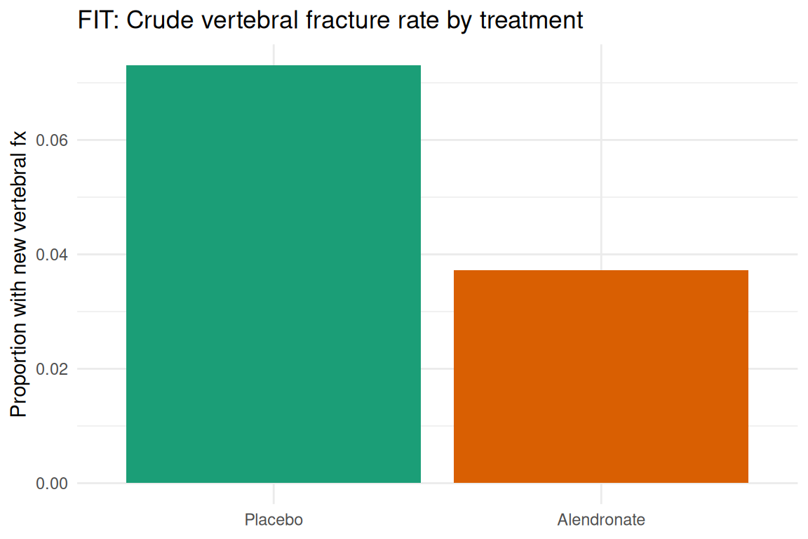
fit_model <- stats::glm(formula_main, data = dat, family = stats::binomial())
summary(fit_model)
#>
#> Call:
#> stats::glm(formula = formula_main, family = stats::binomial(),
#>     data = dat)
#>
#> Coefficients:
#>             Estimate Std. Error z value Pr(>|z|)
#> (Intercept) -4.54016    1.04820  -4.331 1.48e-05 ***
#> treat       -0.74296    0.13023  -5.705 1.16e-08 ***
#> age          0.06572    0.01158   5.673 1.40e-08 ***
#> frac_base    1.23173    0.13294   9.266  < 2e-16 ***
#> bmd_base    -0.35406    0.05890  -6.011 1.84e-09 ***
#> ---
#> Signif. codes:  0 '***' 0.001 '**' 0.01 '*' 0.05 '.' 0.1 ' ' 1
#>
#> (Dispersion parameter for binomial family taken to be 1)
#>
#>     Null deviance: 2274.5  on 5323  degrees of freedom
#> Residual deviance: 1993.8  on 5319  degrees of freedom
#> AIC: 2003.8
#>
#> Number of Fisher Scoring iterations: 6fit_unadj <- stats::glm(newvfx ~ treat, data = dat, family = stats::binomial())
stats::anova(fit_unadj, fit_model, test = "Chisq")
#> Analysis of Deviance Table
#>
#> Model 1: newvfx ~ treat
#> Model 2: newvfx ~ treat + age + frac_base + bmd_base
#> Resid. Df Resid. Dev Df Deviance Pr(>Chi)
#> 1 5322 2241.3
#> 2 5319 1993.8 3 247.54 < 2.2e-16 ***
#> ---
#> Signif. codes: 0 '***' 0.001 '**' 0.01 '*' 0.05 '.' 0.1 ' ' 1or <- exp(stats::coef(fit_model))
ci <- exp(stats::confint(fit_model))
data.frame(
term = names(or),
odds_ratio = unname(or),
conf_low = ci[, 1],
conf_high = ci[, 2],
p_value = summary(fit_model)$coefficients[, "Pr(>|z|)"]
)
#> term odds_ratio conf_low conf_high p_value
#> (Intercept) (Intercept) 0.01067166 0.001350607 0.08236414 1.481647e-05
#> treat treat 0.47570534 0.367351009 0.61239533 1.164759e-08
#> age age 1.06792402 1.044124872 1.09265568 1.404115e-08
#> frac_base frac_base 3.42716051 2.647038329 4.45971891 1.940830e-20
#> bmd_base bmd_base 0.70183113 0.625168747 0.78763335 1.839665e-09Alendronate treatment is associated with substantially reduced odds of new vertebral fracture compared to placebo after adjustment for baseline fracture history, BMD, and age, replicating the main finding of Black et al. (1996) and discussed in RMB2e Chapter 6. Prior vertebral fracture and lower baseline BMD are both strong independent predictors of incident fracture, confirming their roles as established risk factors. These results illustrate how logistic regression can estimate treatment effects adjusted for important prognostic baseline characteristics in a randomized trial.