HERS data

This article reproduces HERS analyses from RMB2e Chapters 3 and 4, examining BMI–LDL associations and the interaction between hormone therapy and statin use.

1 Introduction

The Heart and Estrogen/Progestin Replacement Study (HERS) was a randomized controlled trial enrolling postmenopausal women with established coronary heart disease to evaluate whether hormone therapy (HT) reduced cardiovascular events. Beyond its primary endpoint, HERS provides rich baseline and follow-up data for studying lipid outcomes and their determinants. Elevated LDL cholesterol is a well-established modifiable risk factor for coronary disease, and understanding its predictors supports both clinical management and study planning.

Code

data(rmb_datasets, package = "rmb")
rmb_datasets$study_design[rmb_datasets$object == "hers"]
#> [1] "Randomized placebo-controlled trial in postmenopausal women with CHD evaluating hormone therapy."

Is higher BMI associated with higher LDL after adjustment for demographic and lifestyle covariates, and does the treatment effect of HT on year-1 LDL differ by baseline statin use?

1.1 Causal assumptions

Code

set.seed(42)
dag <- ggdag::dagify(
  ldl1 ~ ht + statin + int_ht_statin + bmi + age + nw + smk + drink,
  int_ht_statin ~ ht + statin,
  bmi ~ age + nw + smk + drink,
  labels = c(
    ldl1 = "Year-1 LDL",
    ht = "Randomized HT",
    statin = "Baseline statin",
    int_ht_statin = "HT x statin",
    bmi = "BMI",
    age = "Age",
    nw = "Nonwhite ethnicity",
    smk = "Smoking",
    drink = "Alcohol use"
  ),
  exposure = "ht",
  outcome = "ldl1"
)
ggdag::ggdag(dag, use_labels = "label", text = FALSE) +
  ggdag::theme_dag_blank() +
  ggplot2::labs(title = "HERS: Causal DAG")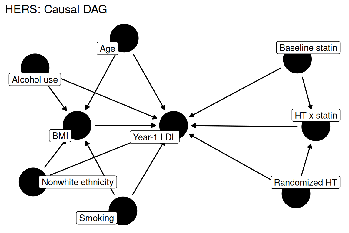

2 Methods

2.1 Study sample

Code

data(hers, package = "rmb")
dat <- haven::zap_labels(hers)
dim(dat)
#> [1] 2763   37
nd <- subset(dat, diabetes == 0)
summary(nd[c("HT", "BMI", "LDL", "LDL1", "exercise", "glucose", "age", "nonwhite", "smoking", "drinkany", "statins")])
#>        HT              BMI             LDL             LDL1      
#>  Min.   :0.0000   Min.   :15.21   Min.   : 36.8   Min.   : 36.8  
#>  1st Qu.:0.0000   1st Qu.:24.20   1st Qu.:120.6   1st Qu.:107.6  
#>  Median :0.0000   Median :26.89   Median :141.4   Median :129.6  
#>  Mean   :0.4926   Mean   :27.67   Mean   :145.6   Mean   :133.2  
#>  3rd Qu.:1.0000   3rd Qu.:30.27   3rd Qu.:166.0   3rd Qu.:154.2  
#>  Max.   :1.0000   Max.   :54.13   Max.   :351.2   Max.   :340.0  
#>                   NAs    :2       NAs    :7       NAs    :100    
#>     exercise         glucose            age           nonwhite      
#>  Min.   :0.0000   Min.   : 47.00   Min.   :44.00   Min.   :0.00000  
#>  1st Qu.:0.0000   1st Qu.: 90.00   1st Qu.:62.00   1st Qu.:0.00000  
#>  Median :0.0000   Median : 96.00   Median :67.00   Median :0.00000  
#>  Mean   :0.4139   Mean   : 96.66   Mean   :66.89   Mean   :0.08661  
#>  3rd Qu.:1.0000   3rd Qu.:102.00   3rd Qu.:72.00   3rd Qu.:0.00000  
#>  Max.   :1.0000   Max.   :125.00   Max.   :79.00   Max.   :1.00000  
#>                                                                     
#>     smoking          drinkany         statins      
#>  Min.   :0.0000   Min.   :0.0000   Min.   :0.0000  
#>  1st Qu.:0.0000   1st Qu.:0.0000   1st Qu.:0.0000  
#>  Median :0.0000   Median :0.0000   Median :0.0000  
#>  Mean   :0.1471   Mean   :0.4409   Mean   :0.3711  
#>  3rd Qu.:0.0000   3rd Qu.:1.0000   3rd Qu.:1.0000  
#>  Max.   :1.0000   Max.   :1.0000   Max.   :1.0000  
#>                   NAs    :2

2.2 Statistical analysis

Two linear models are fitted: Model A (RMB2e p. 113) regresses LDL on BMI adjusted for age, race/ethnicity, smoking, and alcohol in the non-diabetic subsample; Model B (RMB2e pp. 120–121) tests the HT × statin interaction for year-1 LDL in the full cohort.

Code

formula_bmi_ldl <- LDL ~ BMI + age + nonwhite + smoking + drinkany
formula_ht_statin <- LDL1 ~ HT * statins

list(
  bmi_ldl_model = formula_bmi_ldl,
  ht_statin_model = formula_ht_statin
)
#> $bmi_ldl_model
#> LDL ~ BMI + age + nonwhite + smoking + drinkany
#> 
#> $ht_statin_model
#> LDL1 ~ HT * statins

3 Results

3.1 Descriptive statistics

Code

with(nd, tapply(glucose, exercise, summary))
#> $`0`
#>    Min. 1st Qu.  Median    Mean 3rd Qu.    Max. 
#>   67.00   90.00   96.00   97.36  103.00  125.00 
#> 
#> $`1`
#>    Min. 1st Qu.  Median    Mean 3rd Qu.    Max. 
#>   47.00   89.00   95.00   95.67  101.00  125.00
stats::t.test(glucose ~ exercise, data = nd)
#> 
#>  Welch Two Sample t-test
#> 
#> data:  glucose by exercise
#> t = 3.8995, df = 1858.3, p-value = 9.984e-05
#> alternative hypothesis: true difference in means between group 0 and group 1 is not equal to 0
#> 95 percent confidence interval:
#>  0.8413953 2.5441828
#> sample estimates:
#> mean in group 0 mean in group 1 
#>        97.36104        95.66825

summary(nd$BMI)
#>    Min. 1st Qu.  Median    Mean 3rd Qu.    Max.     NAs 
#>   15.21   24.20   26.89   27.67   30.27   54.13       2
summary(nd$LDL)
#>    Min. 1st Qu.  Median    Mean 3rd Qu.    Max.     NAs 
#>    36.8   120.6   141.4   145.6   166.0   351.2       7
with(nd, cor(BMI, LDL, use = "complete.obs"))
#> [1] 0.08079376

Code

ggplot2::ggplot(nd, ggplot2::aes(x = BMI, y = LDL)) +
  ggplot2::geom_point(alpha = 0.2, size = 1) +
  ggplot2::geom_smooth(method = "lm", se = FALSE, color = "#d95f02", linewidth = 1) +
  ggplot2::labs(
    title = "HERS: LDL vs BMI (women without diabetes)",
    x = expression("BMI (kg/m"^2*")"),
    y = "LDL (mg/dL)"
  ) +
  ggplot2::theme_minimal()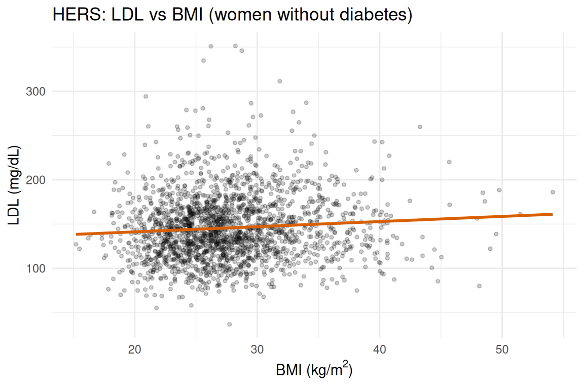

3.2 Model estimates

Code

fit_bmi_ldl <- stats::lm(formula_bmi_ldl, data = nd)
fit_ht_statin <- stats::lm(formula_ht_statin, data = dat)

summary(fit_bmi_ldl)
#> 
#> Call:
#> stats::lm(formula = formula_bmi_ldl, data = nd)
#> 
#> Residuals:
#>      Min       1Q   Median       3Q      Max 
#> -111.364  -24.982   -3.977   20.765  201.167 
#> 
#> Coefficients:
#>             Estimate Std. Error t value Pr(>|t|)    
#> (Intercept) 146.8359    10.5300  13.945  < 2e-16 ***
#> BMI           0.5329     0.1626   3.278  0.00106 ** 
#> age          -0.2361     0.1276  -1.850  0.06453 .  
#> nonwhite      4.9122     2.9547   1.663  0.09656 .  
#> smoking       5.5834     2.4002   2.326  0.02010 *  
#> drinkany     -3.0682     1.6726  -1.834  0.06674 .  
#> ---
#> Signif. codes:  0 '***' 0.001 '**' 0.01 '*' 0.05 '.' 0.1 ' ' 1
#> 
#> Residual standard error: 36.85 on 2015 degrees of freedom
#>   (11 observations deleted due to missingness)
#> Multiple R-squared:  0.01554,    Adjusted R-squared:  0.01309 
#> F-statistic:  6.36 on 5 and 2015 DF,  p-value: 7.217e-06
summary(fit_ht_statin)
#> 
#> Call:
#> stats::lm(formula = formula_ht_statin, data = dat)
#> 
#> Residuals:
#>      Min       1Q   Median       3Q      Max 
#> -147.428  -24.678   -3.952   19.843  305.043 
#> 
#> Coefficients:
#>             Estimate Std. Error t value Pr(>|t|)    
#> (Intercept)  145.157      1.326 109.507  < 2e-16 ***
#> HT           -17.728      1.871  -9.477  < 2e-16 ***
#> statins      -13.809      2.152  -6.416 1.65e-10 ***
#> HT:statins     6.244      3.076   2.030   0.0425 *  
#> ---
#> Signif. codes:  0 '***' 0.001 '**' 0.01 '*' 0.05 '.' 0.1 ' ' 1
#> 
#> Residual standard error: 37.91 on 2604 degrees of freedom
#>   (155 observations deleted due to missingness)
#> Multiple R-squared:  0.05722,    Adjusted R-squared:  0.05613 
#> F-statistic: 52.68 on 3 and 2604 DF,  p-value: < 2.2e-16

3.3 Model diagnostics

Code

fit_data <- data.frame(
  fitted = stats::fitted(fit_bmi_ldl),
  residuals = stats::residuals(fit_bmi_ldl),
  std_residuals = stats::rstandard(fit_bmi_ldl)
)

ggplot2::ggplot(fit_data, ggplot2::aes(x = fitted, y = residuals)) +
  ggplot2::geom_point() +
  ggplot2::geom_hline(yintercept = 0, linetype = "dashed", color = "red") +
  ggplot2::geom_smooth(se = FALSE, color = "blue") +
  ggplot2::labs(
    title = "Residuals vs Fitted",
    x = "Fitted values",
    y = "Residuals"
  ) +
  ggplot2::theme_minimal()

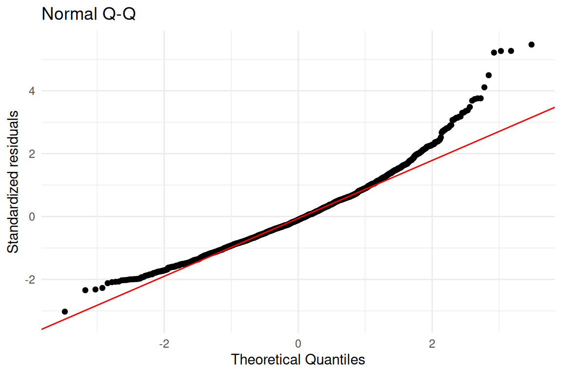
ggplot2::ggplot(fit_data, ggplot2::aes(sample = std_residuals)) +
  ggplot2::stat_qq() +
  ggplot2::stat_qq_line(color = "red") +
  ggplot2::labs(
    title = "Normal Q-Q",
    x = "Theoretical Quantiles",
    y = "Standardized residuals"
  ) +
  ggplot2::theme_minimal()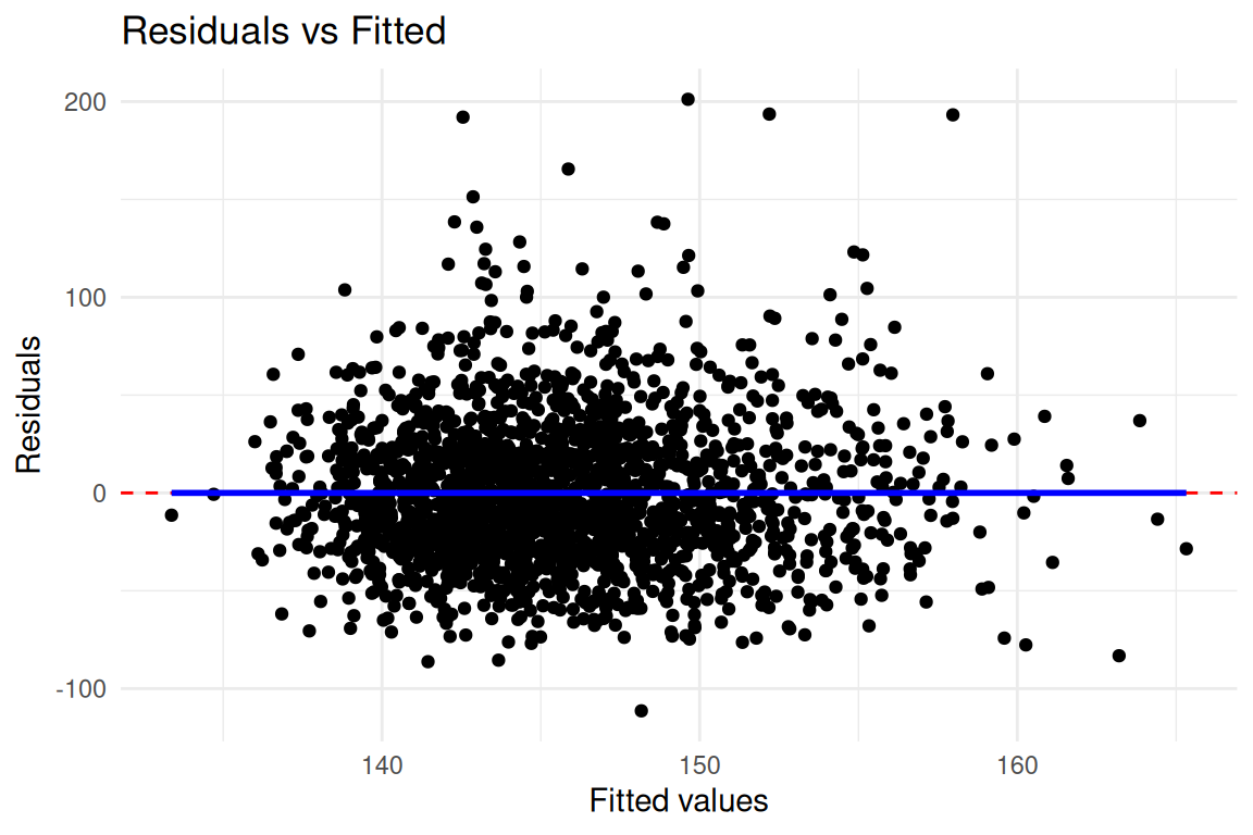

Code

stats::coef(fit_ht_statin)["HT"] + stats::coef(fit_ht_statin)["HT:statins"]
#>        HT 
#> -11.48394

3.4 Inference

Code

ci_bmi <- stats::confint(fit_bmi_ldl)
ci_int <- stats::confint(fit_ht_statin)

inf_bmi <- data.frame(
  term = names(stats::coef(fit_bmi_ldl)),
  estimate = stats::coef(fit_bmi_ldl),
  conf_low = ci_bmi[, 1],
  conf_high = ci_bmi[, 2],
  p_value = summary(fit_bmi_ldl)$coefficients[, "Pr(>|t|)"]
)

inf_int <- data.frame(
  term = names(stats::coef(fit_ht_statin)),
  estimate = stats::coef(fit_ht_statin),
  conf_low = ci_int[, 1],
  conf_high = ci_int[, 2],
  p_value = summary(fit_ht_statin)$coefficients[, "Pr(>|t|)"]
)

inf_bmi
#>                    term    estimate    conf_low    conf_high      p_value
#> (Intercept) (Intercept) 146.8359212 126.1851907 167.48665176 2.922395e-42
#> BMI                 BMI   0.5329454   0.2141127   0.85177810 1.062670e-03
#> age                 age  -0.2360610  -0.4863685   0.01424642 6.452879e-02
#> nonwhite       nonwhite   4.9122153  -0.8823294  10.70675994 9.656391e-02
#> smoking         smoking   5.5834329   0.8763636  10.29050223 2.010299e-02
#> drinkany       drinkany  -3.0682259  -6.3484149   0.21196312 6.673984e-02
inf_int
#>                    term   estimate    conf_low  conf_high      p_value
#> (Intercept) (Intercept) 145.156724 142.5574870 147.755960 0.000000e+00
#> HT                   HT -17.728360 -21.3964301 -14.060290 5.662862e-21
#> statins         statins -13.809124 -18.0291829  -9.589065 1.650947e-10
#> HT:statins   HT:statins   6.244416   0.2118042  12.277028 4.248635e-02

4 Discussion

Higher BMI is associated with higher LDL after adjustment for age, race/ethnicity, smoking, and alcohol (RMB2e p. 113), consistent with the known metabolic coupling between adiposity and dyslipidemia. The effect of hormone therapy on LDL differs by baseline statin use (RMB2e pp. 120–121), illustrating effect modification on the linear-model scale; among statin users the HT benefit on LDL is substantially attenuated, a finding discussed in the context of interaction interpretation in Chapter 4 (p. 126).

5 Source

UCSF Regression Methods companion data: https://regression.ucsf.edu/sites/g/files/tkssra16191/files/wysiwyg/home/data/hersdata.dta
Book: Vittinghoff E, Glidden DV, Shiboski SC, McCulloch CE (2012). Regression Methods in Biostatistics (2nd edition).