ACTG 019 data

This article reproduces the ACTG 019 survival analysis workflow used in RMB2e Chapter 6, estimating the effect of zidovudine on time to AIDS or death.

1 Introduction

The AIDS Clinical Trials Group protocol 019 was a placebo-controlled randomized trial of zidovudine (ZDV) in HIV-positive adults with CD4 counts between 200 and 500 cells/mm³, conducted in the late 1980s. It was among the first trials to demonstrate a survival benefit for antiretroviral therapy in this CD4 stratum. Baseline CD4 count is a strong predictor of disease progression and is included as a covariate to increase precision, even though randomization removes confounding by design (RMB2e p. 268).

Code

data(rmb_datasets, package = "rmb")
rmb_datasets$study_design[rmb_datasets$object == "actg019"]
#> [1] "Randomized double-blind placebo-controlled trial of zidovudine in HIV infection."

Can zidovudine treatment reduce the hazard of AIDS or death after accounting for baseline CD4 cell count?

1.1 Causal assumptions

Code

set.seed(42)
dag <- ggdag::dagify(
  time_aids ~ rx + cd4,
  rx ~ cd4,
  labels = c(
    time_aids = "Time to AIDS/death",
    rx = "ZDV treatment",
    cd4 = "Baseline CD4"
  ),
  exposure = "rx",
  outcome = "time_aids"
)
ggdag::ggdag(dag, use_labels = "label", text = FALSE) +
  ggdag::theme_dag_blank() +
  ggplot2::labs(title = "ACTG 019: Causal DAG")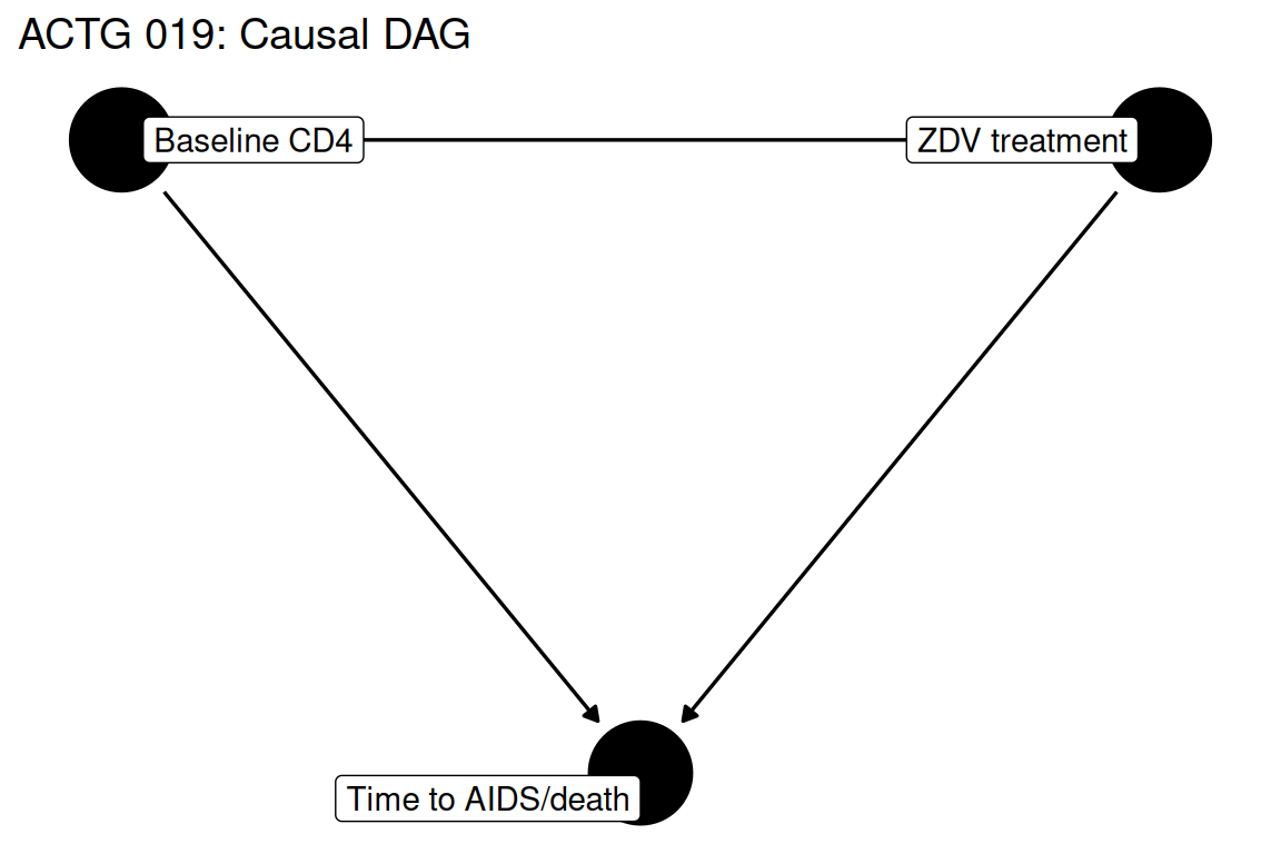

Figure 1: Directed acyclic graph for the ACTG 019 treatment-outcome structure.

2 Methods

2.1 Study sample

Code

data(actg019, package = "rmb")
dat <- actg019
dim(dat)
#> [1] 880   5
summary(haven::zap_labels(dat[c("days", "cens", "rx", "cd4")]))
#>       days            cens              rx              cd4       
#>  Min.   :  1.0   Min.   :0.0000   Min.   :0.0000   Min.   : 30.0  
#>  1st Qu.:234.8   1st Qu.:0.0000   1st Qu.:0.0000   1st Qu.:251.0  
#>  Median :373.0   Median :0.0000   Median :1.0000   Median :343.5  
#>  Mean   :403.3   Mean   :0.0625   Mean   :0.5136   Mean   :332.2  
#>  3rd Qu.:573.0   3rd Qu.:0.0000   3rd Qu.:1.0000   3rd Qu.:420.0  
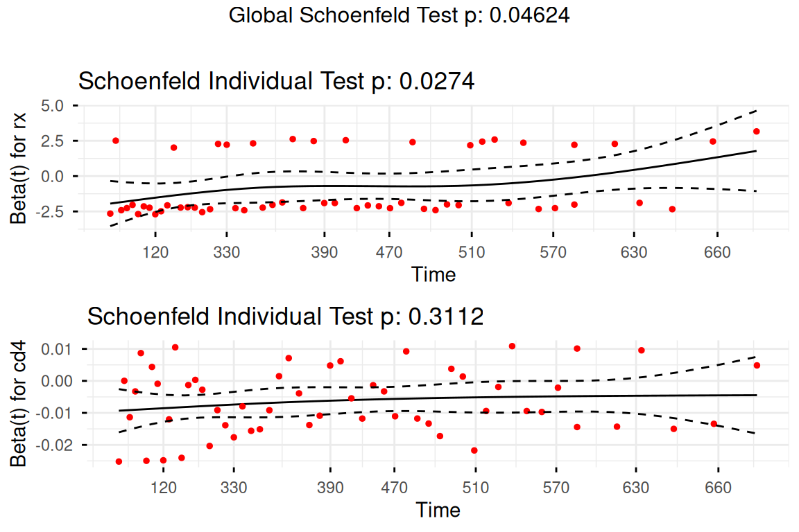
#>  Max.   :746.0   Max.   :1.0000   Max.   :1.0000   Max.   :704.0

2.2 Statistical analysis

A Cox proportional hazards model with Breslow tie-handling is used, regressing the survival outcome on treatment assignment and baseline CD4 count (RMB2e p. 267). The proportional hazards assumption is checked with scaled Schoenfeld residuals.

Code

cox_formula <- survival::Surv(days, cens) ~ rx + cd4
cox_formula
#> survival::Surv(days, cens) ~ rx + cd4

3 Results

3.1 Descriptive statistics

Code

with(dat, c(
  n = length(days),
  n_events = sum(cens == 1, na.rm = TRUE),
  event_rate = mean(cens == 1, na.rm = TRUE),
  median_followup_days = median(days, na.rm = TRUE)
))
#>                    n             n_events           event_rate 
#>             880.0000              55.0000               0.0625 
#> median_followup_days 
#>             373.0000

with(dat, tapply(cd4, rx, summary))
#> $`0`
#>    Min. 1st Qu.  Median    Mean 3rd Qu.    Max. 
#>    30.0   242.0   343.0   332.7   422.0   704.0 
#> 
#> $`1`
#>    Min. 1st Qu.  Median    Mean 3rd Qu.    Max. 
#>    35.0   257.0   343.5   331.8   416.0   500.0
with(dat, tapply(days, rx, summary))
#> $`0`
#>    Min. 1st Qu.  Median    Mean 3rd Qu.    Max. 
#>       1     256     489     425     588     746 
#> 
#> $`1`
#>    Min. 1st Qu.  Median    Mean 3rd Qu.    Max. 
#>     1.0   224.0   338.0   382.7   560.0   743.0

Code

dat$rx_plot <- factor(dat$rx, levels = c(0, 1), labels = c("Placebo", "ZDV"))
km_fit <- survival::survfit(survival::Surv(days, cens) ~ rx_plot, data = dat)

survminer::ggsurvplot(
  km_fit,
  data = dat,
  title = "ACTG 019 Kaplan-Meier curves by treatment",
  xlab = "Days since randomization",
  ylab = "AIDS/death-free survival",
  legend.title = "Treatment",
  ggtheme = ggplot2::theme_minimal(),
  palette = c("#1b9e77", "#d95f02"),
  conf.int = FALSE,
  censor = TRUE
)

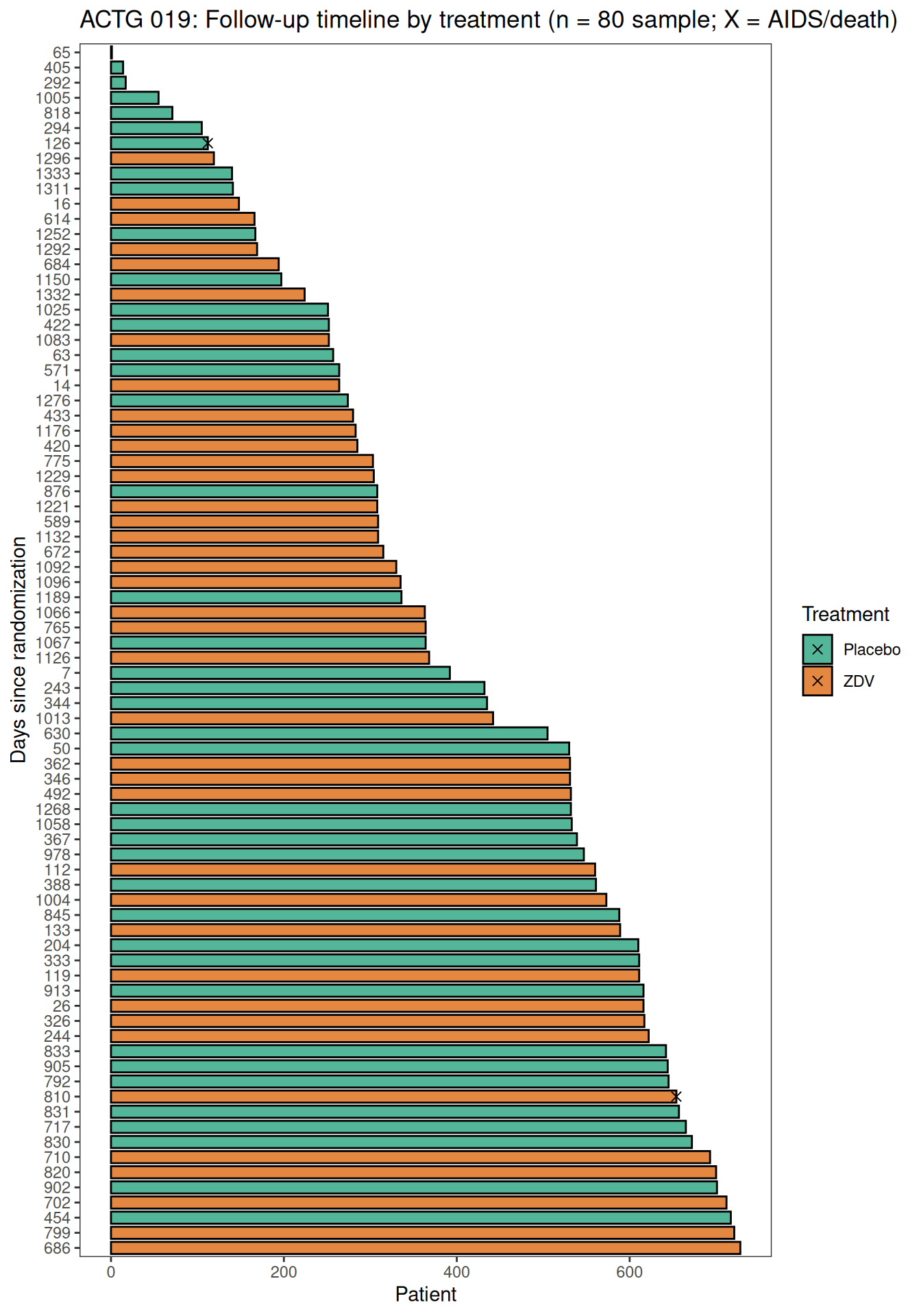
Figure 2: Kaplan-Meier survival curves by randomized treatment arm.

The swimmer plot below shows individual follow-up times for a random sample of 80 participants (40 per arm), with × marks indicating AIDS/death events.

Code

set.seed(42)
dat_swim <- as.data.frame(dat)
dat_swim$days <- as.numeric(dat_swim$days)
dat_swim$rx_int <- as.integer(unclass(dat_swim$rx))
dat_swim$cens_int <- as.integer(unclass(dat_swim$cens))
ids_0 <- sample(dat_swim$id[dat_swim$rx_int == 0], 40)
ids_1 <- sample(dat_swim$id[dat_swim$rx_int == 1], 40)
dat_sub <- dat_swim[dat_swim$id %in% c(ids_0, ids_1), ]
dat_sub$Treatment <- factor(
  dat_sub$rx_int,
  levels = c(0, 1),
  labels = c("Placebo", "ZDV")
)
dat_events <- dat_sub[dat_sub$cens_int == 1, ]

swimplot::swimmer_plot(
  df = dat_sub, id = "id", end = "days",
  name_fill = "Treatment", increasing = FALSE,
  col = "black", alpha = 0.75, width = 0.8
) +
  swimplot::swimmer_points(
    df = dat_events, id = "id", time = "days",
    shape = 4, size = 2, col = "black"
  ) +
  ggplot2::scale_fill_manual(values = c("#1b9e77", "#d95f02")) +
  ggplot2::labs(
    x = "Days since randomization",
    y = "Patient",
    title = "ACTG 019: Follow-up timeline by treatment (n = 80 sample; X = AIDS/death)"
  )

Figure 3: Swimmer plot of follow-up time with event markers in a balanced sample.

3.2 Model estimates

Code

fit_cox <- survival::coxph(cox_formula, data = dat, ties = "breslow")
summary(fit_cox)
#> Call:
#> survival::coxph(formula = cox_formula, data = dat, ties = "breslow")
#> 
#>   n= 880, number of events= 55 
#> 
#>          coef exp(coef)  se(coef)      z Pr(>|z|)    
#> rx  -0.785115  0.456067  0.293052 -2.679  0.00738 ** 
#> cd4 -0.006575  0.993446  0.001238 -5.313 1.08e-07 ***
#> ---
#> Signif. codes:  0 '***' 0.001 '**' 0.01 '*' 0.05 '.' 0.1 ' ' 1
#> 
#>     exp(coef) exp(-coef) lower .95 upper .95
#> rx     0.4561      2.193    0.2568    0.8100
#> cd4    0.9934      1.007    0.9910    0.9959
#> 
#> Concordance= 0.737  (se = 0.034 )
#> Likelihood ratio test= 34.46  on 2 df,   p=3e-08
#> Wald test            = 33.33  on 2 df,   p=6e-08
#> Score (logrank) test = 35.4  on 2 df,   p=2e-08

3.3 Model diagnostics

Code

ph_test <- survival::cox.zph(fit_cox)
ph_test
#>        chisq df     p
#> rx      4.87  1 0.027
#> cd4     1.03  1 0.311
#> GLOBAL  6.15  2 0.046

survminer::ggcoxzph(
  ph_test,
  ggtheme = ggplot2::theme_minimal()
)

Figure 4: Scaled Schoenfeld residual diagnostics for proportional hazards assumptions.

3.4 Inference

Code

hr <- exp(stats::coef(fit_cox))
ci <- exp(stats::confint(fit_cox))
knitr::kable(data.frame(
  term = names(hr),
  hazard_ratio = unname(hr),
  conf_low = ci[, 1],
  conf_high = ci[, 2],
  p_value = summary(fit_cox)$coefficients[, "Pr(>|z|)"]
), digits = 3)

Table 1: Cox model hazard-ratio estimates with 95% confidence intervals and p-values.

	term	hazard_ratio	conf_low	conf_high	p_value
rx	rx	0.456	0.257	0.810	0.007
cd4	cd4	0.993	0.991	0.996	0.000

4 Discussion

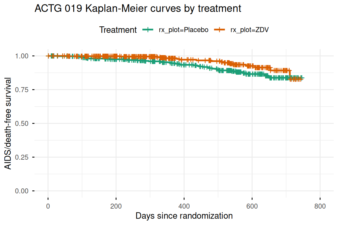
ZDV assignment is associated with a lower hazard of AIDS or death, consistent with the trial’s primary findings as discussed in RMB2e Chapter 6 (pp. 224, 267). Higher baseline CD4 count is protective, reflecting the well-known relationship between immune status and disease progression. The proportional hazards assumption diagnostics (Schoenfeld residuals) should be inspected to confirm that hazard ratios are constant over follow-up time, a key requirement for valid Cox model interpretation (RMB2e p. 267).

5 Source

UCSF Regression Methods companion data: https://regression.ucsf.edu/sites/g/files/tkssra16191/files/wysiwyg/home/data/actg019.dta
Book: Vittinghoff E, Glidden DV, Shiboski SC, McCulloch CE (2012). Regression Methods in Biostatistics (2nd edition).