Nonparametric Models

---

Configuring R

Functions from these packages will be used throughout this document:

library(conflicted) # check for conflicting function definitions
# library(printr) # inserts help-file output into markdown output
library(rmarkdown) # Convert R Markdown documents into a variety of formats.
library(pander) # format tables for markdown
library(ggplot2) # graphics
library(ggfortify) # help with graphics
library(dplyr) # manipulate data
library(tibble) # `tibble`s extend `data.frame`s
library(magrittr) # `%>%` and other additional piping tools
library(haven) # import Stata files
library(knitr) # format R output for markdown
library(tidyr) # Tools to help to create tidy data
library(plotly) # interactive graphics
library(dobson) # datasets from Dobson and Barnett 2018
library(parameters) # format model output tables for markdown
library(haven) # import Stata files
library(latex2exp) # use LaTeX in R code (for figures and tables)
library(fs) # filesystem path manipulations
library(survival) # survival analysis
library(survminer) # survival analysis graphics
library(KMsurv) # datasets from Klein and Moeschberger
library(parameters) # format model output tables for
library(webshot2) # convert interactive content to static for pdf
library(forcats) # functions for categorical variables ("factors")
library(stringr) # functions for dealing with strings
library(lubridate) # functions for dealing with dates and times
library(broom) # Summarizes key information about statistical objects in tidy tibbles
library(broom.helpers) # Provides suite of functions to work with regression model 'broom::tidy()' tibbles

Here are some R settings I use in this document:

rm(list = ls()) # delete any data that's already loaded into R

conflicts_prefer(dplyr::filter)
ggplot2::theme_set(
  ggplot2::theme_bw() + 
        # ggplot2::labs(col = "") +
    ggplot2::theme(
      legend.position = "bottom",
      text = ggplot2::element_text(size = 12, family = "serif")))

knitr::opts_chunk$set(message = FALSE)
options('digits' = 6)

panderOptions("big.mark", ",")
pander::panderOptions("table.emphasize.rownames", FALSE)
pander::panderOptions("table.split.table", Inf)
conflicts_prefer(dplyr::filter) # use the `filter()` function from dplyr() by default
legend_text_size = 9
run_graphs = TRUE

---

1 Empirical CDF and quantiles

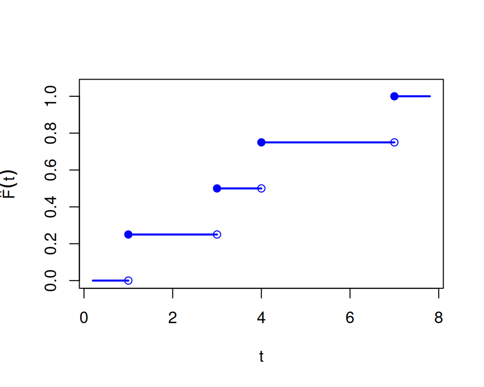
Definition 1 (Empirical CDF) For observed values \(x_1,\ldots,x_n\), the empirical CDF is \[\hat F(t)=\frac{1}{n}\sum_{j=1}^n I(x_j\le t), \quad t\in\mathbb{R}.\] Here \(I(A)\) is the indicator function: \(I(A)=1\) if \(A\) holds, and \(I(A)=0\) otherwise.

Definition 2 (Order statistics) For observed values \(x_1,\ldots,x_n\), the order statistics are the sorted values \[x_{(1)}\le x_{(2)}\le\cdots\le x_{(n)}.\]

Example 1 (Numerical example: order statistics) If the observed values are \(4,1,7,3\), then the order statistics are \(x_{(1)}=1\), \(x_{(2)}=3\), \(x_{(3)}=4\), and \(x_{(4)}=7\).

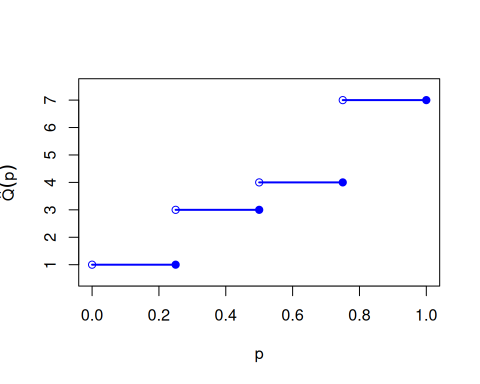
Definition 3 (Sample quantile) Given empirical CDF \(\hat F\), the sample quantile function (EQF) (the generalized inverse of \(\hat F\)) is \[\hat Q(p)=\inf\{t:\hat F(t)\ge p\}, \quad 0<p\le 1.\]

The CDF \(F\) and quantile function \(Q\) are population-level functions, while \(\hat F\) and \(\hat Q\) are sample-based estimates of them.

Theorem 1 (Order-statistics form of the sample quantile) If \(x_{(1)}\le\cdots\le x_{(n)}\) are the order statistics, then \(\hat Q(p)=x_{(i)}\) for \(p\in((i-1)/n,i/n]\). In particular, \(\hat Q(i/n)=x_{(i)}\).

Example 2 (Numerical example: sample quantiles) Using the same data \(4,1,7,3\), with order statistics \(1,3,4,7\), the sample quantile function is stepwise: \(\hat Q(p)=1\) for \(0<p\le 1/4\), \(\hat Q(p)=3\) for \(1/4<p\le 1/2\), \(\hat Q(p)=4\) for \(1/2<p\le 3/4\), and \(\hat Q(p)=7\) for \(3/4<p\le 1\). So \(\hat Q(0.5)=3\) and \(\hat Q(0.9)=7\).

x <- c(4, 1, 7, 3)
n <- length(x)
x_ord <- sort(x)
p_ord <- seq_len(n) / n
ecdf_x_padding <- 0.8
eqf_y_padding <- 0.5
x_min <- min(x_ord) - ecdf_x_padding
x_max <- max(x_ord) + ecdf_x_padding

x_left <- c(x_min, x_ord)
x_right <- c(x_ord, x_max)
f_levels <- c(0, p_ord)

plot(
  0,
  0,
  type = "n",
  xlim = c(x_min, x_max),
  ylim = c(0, 1.05),
  xlab = "t",
  ylab = expression(hat(plain("F"))(t))
)
segments(x_left, f_levels, x_right, f_levels, lwd = 2, col = "blue")
points(x_ord, f_levels[seq_len(n)], pch = 1, col = "blue")
points(x_ord, f_levels[seq_len(n) + 1], pch = 19, col = "blue")

q_left <- c(0, p_ord[-n])
q_right <- p_ord
plot(
  0,
  0,
  type = "n",
  xlim = c(0, 1),
  ylim = c(min(x_ord) - eqf_y_padding, max(x_ord) + eqf_y_padding),
  xlab = "p",
  ylab = expression(hat(Q)(p))
)
segments(q_left, x_ord, q_right, x_ord, lwd = 2, col = "blue")
points(q_left, x_ord, pch = 1, col = "blue")
points(q_right, x_ord, pch = 19, col = "blue")

Figure 1: Relationship between the empirical CDF and sample quantiles for data 4, 1, 7, 3. (Order statistics are 1, 3, 4, 7.)

(a) Empirical CDF horizontal pieces only. Closed circles mark included endpoints. Open circles mark excluded endpoints.

(b) Sample quantile function horizontal pieces only. Open circles mark excluded left endpoints. Closed circles mark included right endpoints.

Because both functions are step functions, they are not one-to-one. Flat regions in one function map many inputs to the same output, and jump points in one correspond to intervals in the other. So they are generalized inverses rather than exact two-sided inverses.