6  Introduction to Survival Analysis

---

Configuring R

Functions from these packages will be used throughout this document:

library(conflicted) # check for conflicting function definitions
# library(printr) # inserts help-file output into markdown output
library(rmarkdown) # Convert R Markdown documents into a variety of formats.
library(pander) # format tables for markdown
library(ggplot2) # graphics
library(ggeasy) # help with graphics
library(ggfortify) # help with graphics
library(dplyr) # manipulate data
library(tibble) # `tibble`s extend `data.frame`s
library(magrittr) # `%>%` and other additional piping tools
library(haven) # import Stata files
library(knitr) # format R output for markdown
library(tidyr) # Tools to help to create tidy data
library(plotly) # interactive graphics
library(dobson) # datasets from Dobson and Barnett 2018
library(parameters) # format model output tables for markdown
library(haven) # import Stata files
library(latex2exp) # use LaTeX in R code (for figures and tables)
library(fs) # filesystem path manipulations
library(survival) # survival analysis
library(survminer) # survival analysis graphics
library(KMsurv) # datasets from Klein and Moeschberger
library(parameters) # format model output tables for
library(webshot2) # convert interactive content to static for pdf
library(forcats) # functions for categorical variables ("factors")
library(stringr) # functions for dealing with strings
library(lubridate) # functions for dealing with dates and times

Here are some R settings I use in this document:

rm(list = ls()) # delete any data that's already loaded into R

conflicts_prefer(dplyr::filter)
ggplot2::theme_set(
  ggplot2::theme_bw() + 
        # ggplot2::labs(col = "") +
    ggplot2::theme(
      legend.position = "bottom",
      text = ggplot2::element_text(size = 12, family = "serif")))

knitr::opts_chunk$set(message = FALSE)
options('digits' = 4)

panderOptions("big.mark", ",")
pander::panderOptions("table.emphasize.rownames", FALSE)
pander::panderOptions("table.split.table", Inf)
conflicts_prefer(dplyr::filter) # use the `filter()` function from dplyr() by default
legend_text_size = 9

6.1 Overview

6.1.1 Time-to-event outcomes

Survival analysis is a framework for modeling time-to-event outcomes. It is used in:

• clinical trials, where the event is often death or recurrence of disease.
• engineering reliability analysis, where the event is failure of a device or system.
• insurance, particularly life insurance, where the event is death.

Note

The term survival analysis is a bit misleading. Survival outcomes can sometimes be analyzed using binomial models (logistic regression). Time-to-event models or survival time analysis might be a better name.

6.2 Time-to-event outcome distributions

6.2.1 Distributions of Time-to-Event Data

• The distribution of event times is asymmetric and can be long-tailed, and starts at 0 (that is, \(P(T<0) = 0\)).
• The base distribution is not normal, but exponential.
• There are usually censored observations, which are ones in which the failure time is not observed.
• Often, these are right-censored, meaning that we know that the event occurred after some known time \(t\), but we don’t know the actual event time, as when a patient is still alive at the end of the study.
• Observations can also be left-censored, meaning we know the event has already happened at time \(t\), or interval-censored, meaning that we only know that the event happened between times \(t_1\) and \(t_2\).
• Analysis is difficult if censoring is associated with treatment.

6.2.2 Right Censoring

• Patients are in a clinical trial for cancer, some on a new treatment and some on standard of care.
• Some patients in each group have died by the end of the study. We know the survival time (measured for example from time of diagnosis—each person on their own clock).
• Patients still alive at the end of the study are right censored.
• Patients who are lost to follow-up or withdraw from the study may be right-censored.

6.2.3 Left and Interval Censoring

• An individual tests positive for HIV.
• If the event is infection with HIV, then we only know that it has occurred before the testing time \(t\), so this is left censored.
• If an individual has a negative HIV test at time \(t_1\) and a positive HIV test at time \(t_2\), then the infection event is interval censored.

6.3 Distribution functions for time-to-event variables

6.3.1 The Probability Density Function (PDF)

For a time-to-event variable \(T\) with a continuous distribution, the probability density function is defined as usual (see Section C.4.1).

In most time-to-event models, this density is assumed to be 0 for all \(t<0\); that is, \(f(t) = 0, \forall t<0\). In other words, the support of \(T\) is typically \([0,\infty)\).

---

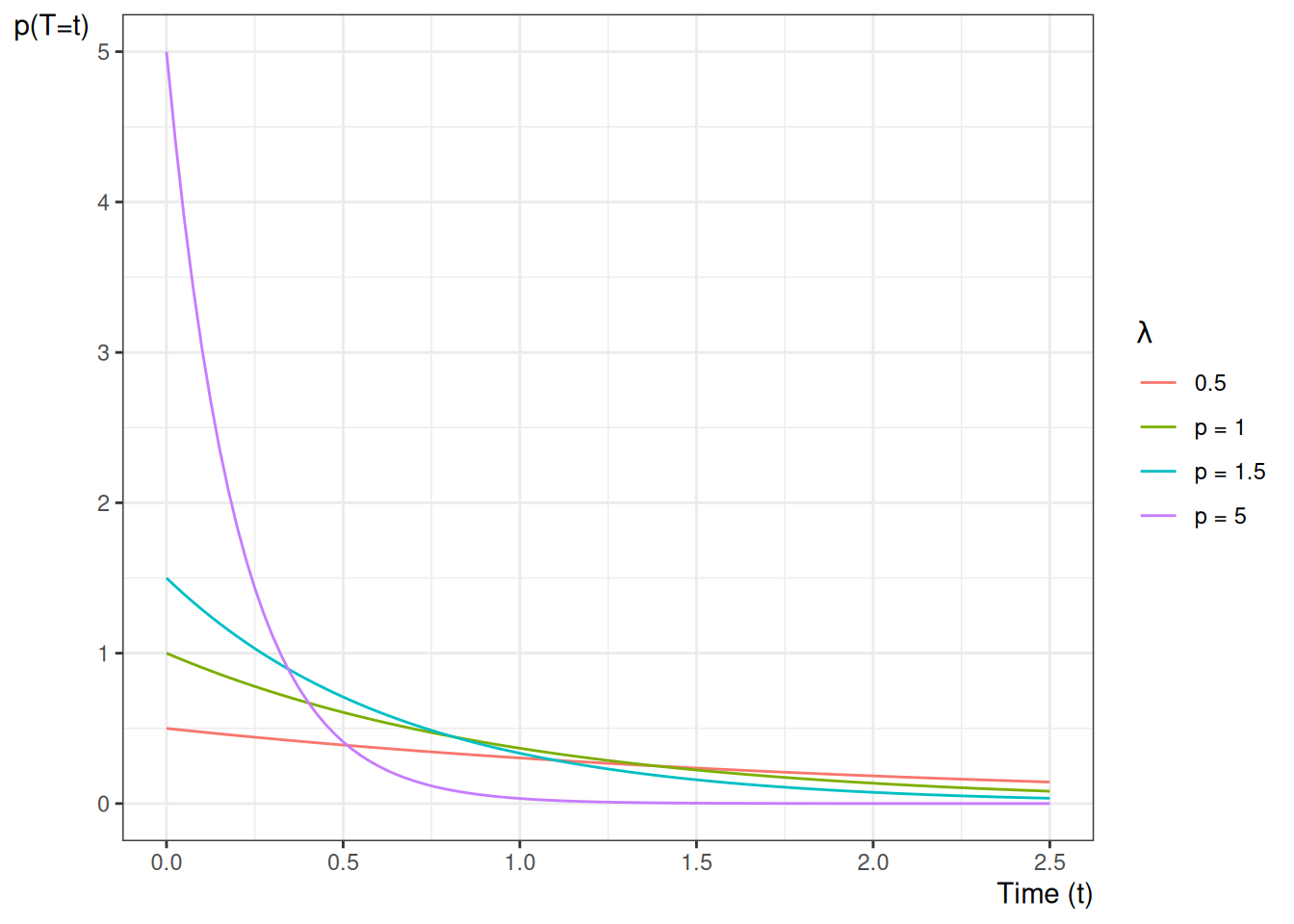
Example 6.1 (exponential distribution) Recall from Epi 202: the pdf of the exponential distribution family of models is:

\[p(T=t) = \mathbb{1}_{t \ge 0} \cdot \lambda \text{e}^{-\lambda t}\]

where \(\lambda > 0\).

---

Here are some examples of exponential pdfs:

6.3.2 The Cumulative Distribution Function (CDF)

The cumulative distribution function is defined as:

\[ \begin{aligned} F(t) &\stackrel{\text{def}}{=}\Pr(T \le t)\\ &=\int_{u=-\infty}^t f(u) du \end{aligned} \]

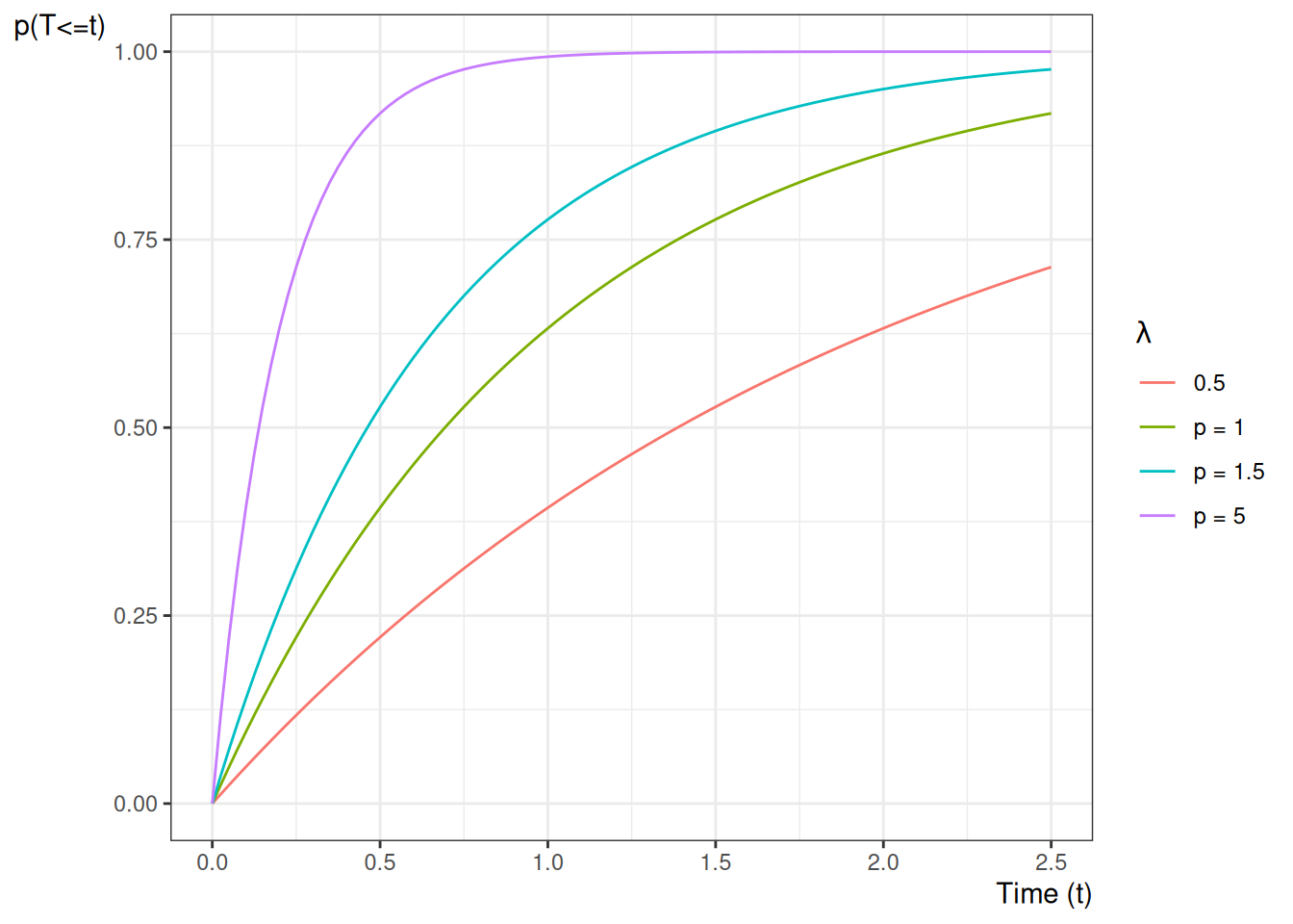
Example 6.2 (exponential distribution) Recall from Epi 202: the cdf of the exponential distribution family of models is:

\[ P(T\le t) = \mathbb{1}_{t \ge 0} \cdot (1- \text{e}^{-\lambda t}) \] where \(\lambda > 0\).

Here are some examples of exponential cdfs:

6.3.3 The Survival Function

For survival data, a more important quantity is the survival function:

\[ \begin{aligned} S(t) &\stackrel{\text{def}}{=}\Pr(T > t)\\ &=\int_{u=t}^\infty p(u) du\\ &=1-F(t)\\ \end{aligned} \]

---

Definition 6.1 (Survival function)  

Given a random time-to-event variable \(T\), the survival function or survivor function, denoted \(S(t)\), is the probability that the event time is later than \(t\). If the event in a clinical trial is death, then \(S(t)\) is the expected fraction of the original population at time 0 who have survived up to time \(t\) and are still alive at time \(t\); that is:

\[S(t) \stackrel{\text{def}}{=}\Pr(T > t) \tag{6.1}\]

---

Example 6.3 (exponential distribution) Since \(S(t) = 1 - F(t)\), the survival function of the exponential distribution family of models is:

\[ P(T> t) = \left\{ {{\text{e}^{-\lambda t}, t\ge0} \atop {1, t \le 0}}\right. \] where \(\lambda > 0\).

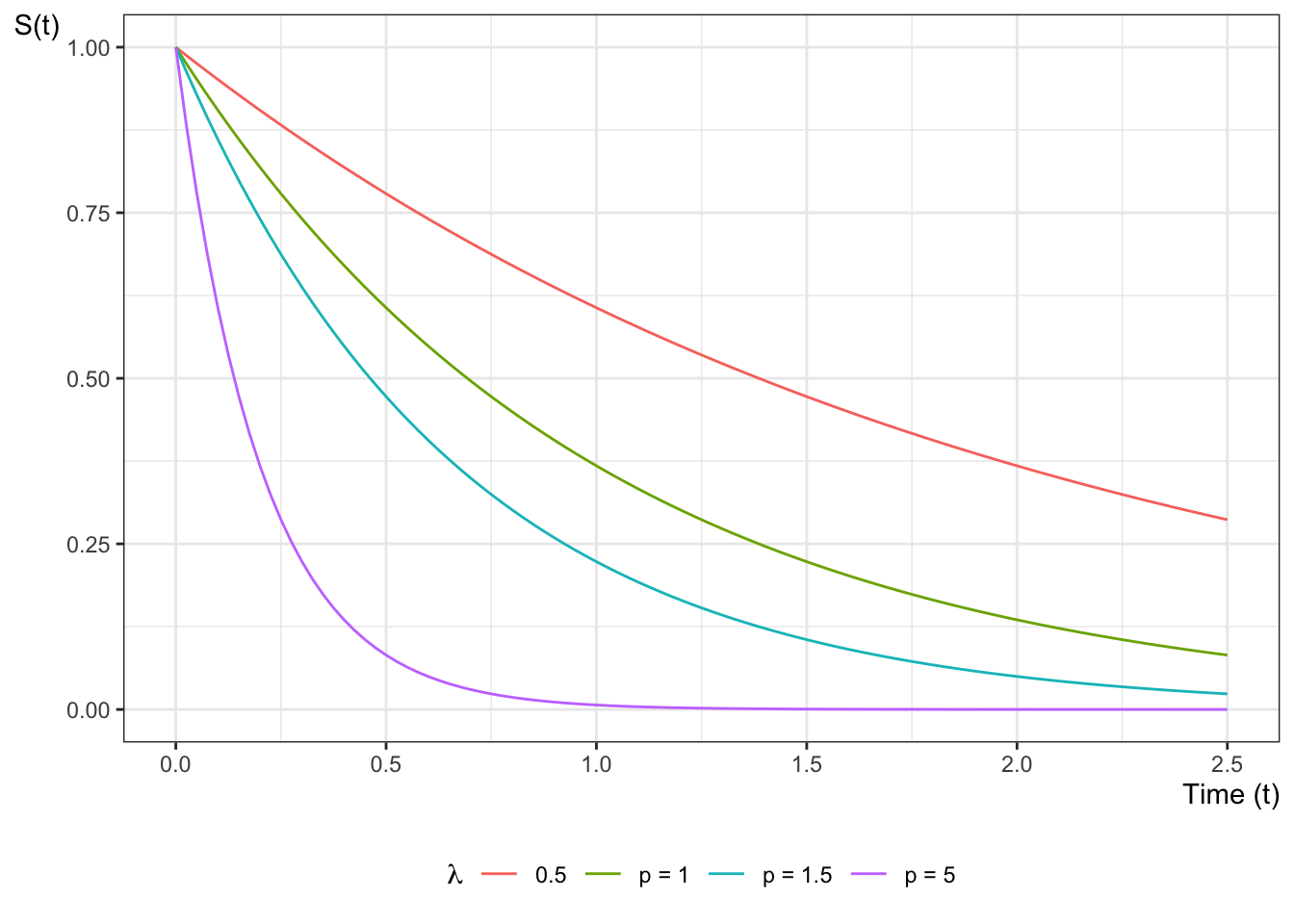
Figure 6.1 shows some examples of exponential survival functions.

---

Figure 6.1: Exponential Survival Functions

---

Theorem 6.1 If \(A_t\) represents survival status at time \(t\), with \(A_t = 1\) denoting alive at time \(t\) and \(A_t = 0\) denoting deceased at time \(t\), then:

\[S(t) = \Pr(A_t=1) = \mathbb{E}[A_t]\]

---

Theorem 6.2 If \(T\) is a nonnegative random variable, then:

\[\mathbb{E}[T] = \int_{t=0}^{\infty} S(t)dt\]

---

Proof. See https://statproofbook.github.io/P/mean-nnrvar.html or

6.3.4 The Hazard Function

Another important quantity is the hazard function:

Definition 6.2 (Hazard function, hazard rate, hazard rate function)  

The hazard function, hazard rate, hazard rate function, for a random variable \(T\) at value \(t\), typically denoted as \(h(t)\) or \(\lambda(t)\), is the conditional density of \(T\) at \(t\), given \(T \ge t\). That is:

\[h(t) \stackrel{\text{def}}{=}\text{p}(T=t|T\ge t)\]

If \(T\) represents the time at which an event occurs, then \(h(t)\) is the probability that the event occurs at time \(t\), given that it has not occurred prior to time \(t\).

---

New content for 2025:

Definition 6.3 (Incidence rate) Given a population of individuals indexed by \(i\), each with their own hazard rate \(h_i(t)\), the incidence rate for that population is the mean hazard rate:

\[\bar{h}(t) \stackrel{\text{def}}{=}\frac{1}{n}\sum_{i=1}^nh_i(t)\]

---

New content for 2025:

Theorem 6.3 (Incidence rate in a homogenous population) If a population of individuals indexed by \(i\) all have identical hazard rates \(h_i(t) = h(t)\), then the incidence rate for that population is equal to the hazard rate:

\[\bar{h}(t) = h(t)\]

(End of new content for 2025)

---

The hazard function has an important relationship to the density and survival functions, which we can use to derive the hazard function for a given probability distribution (Theorem 6.4).

Lemma 6.1 (Joint probability of a variable with itself) \[p(T=t, T\ge t) = p(T=t)\]

Proof. Recall from Epi 202: if \(A\) and \(B\) are statistical events and \(A\subseteq B\), then \(p(A, B) = p(A)\). In particular, \(\{T=t\} \subseteq \{T\geq t\}\), so \(p(T=t, T\ge t) = p(T=t)\).

---

Theorem 6.4 (Hazard equals density over survival) \[h(t)=\frac{f(t)}{S(t)}\]

---

Proof. \[ \begin{aligned} h(t) &=p(T=t|T\ge t)\\ &=\frac{p(T=t, T\ge t)}{p(T \ge t)}\\ &=\frac{p(T=t)}{p(T \ge t)}\\ &=\frac{f(t)}{S(t)} \end{aligned} \]

---

Example 6.4 (exponential distribution) The hazard function of the exponential distribution family of models is:

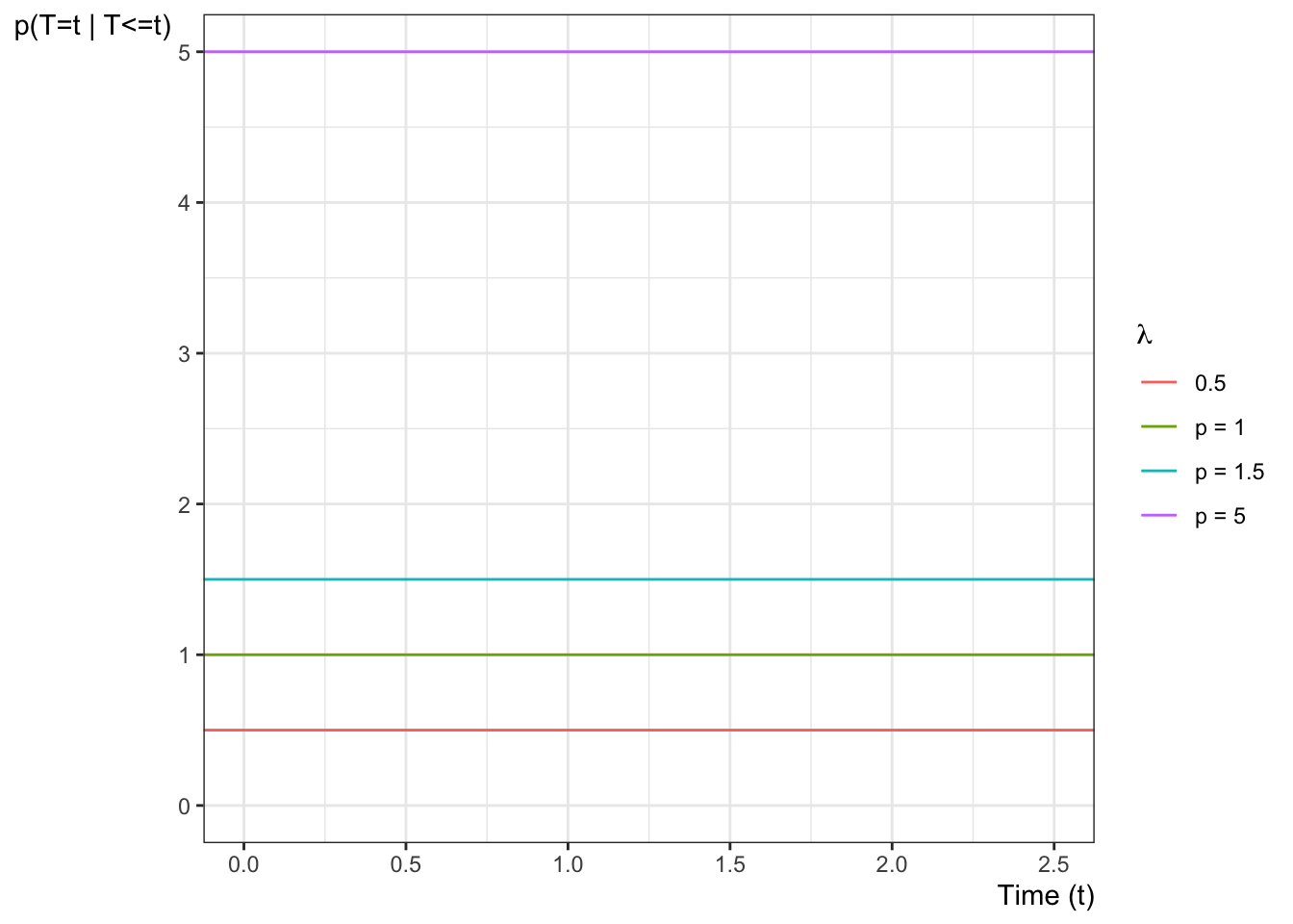
\[ \begin{aligned} P(T=t|T \ge t) &= \frac{f(t)}{S(t)}\\ &= \frac{\mathbb{1}_{t \ge 0}\cdot \lambda \text{e}^{-\lambda t}}{\text{e}^{-\lambda t}}\\ &=\mathbb{1}_{t \ge 0}\cdot \lambda \end{aligned} \] Figure 6.2 shows some examples of exponential hazard functions.

---

Figure 6.2: Examples of hazard functions for exponential distributions

---

We can also view the hazard function as the derivative of the negative of the logarithm of the survival function:

Theorem 6.5 (transform survival to hazard) \[h(t) = \frac{\partial}{\partial t}\left\{-\text{log}\left\{S(t)\right\}\right\}\]

---

Proof. \[ \begin{aligned} h(t) &= \frac{f(t)}{S(t)}\\ &= \frac{-S'(t)}{S(t)}\\ &= -\frac{S'(t)}{S(t)}\\ &=-\frac{\partial}{\partial t}\text{log}\left\{S(t)\right\}\\ &=\frac{\partial}{\partial t}\left\{-\text{log}\left\{S(t)\right\}\right\} \end{aligned} \]

6.3.5 The Cumulative Hazard Function

Since \(h(t) = \frac{\partial}{\partial t}\left\{-\text{log}\left\{S(t)\right\}\right\}\) (see Theorem 6.5), we also have:

Corollary 6.1 \[S(t) = \text{exp}\left\{-\int_{u=0}^t h(u)du\right\} \tag{6.2}\]

---

The integral in Equation 6.2 is important enough to have its own name: cumulative hazard.

Definition 6.4 (cumulative hazard) The cumulative hazard function \(H(t)\) is defined as:

\[H(t) \stackrel{\text{def}}{=}\int_{u=0}^t h(u) du\]

As we will see below, \(H(t)\) is tractable to estimate, and we can then derive an estimate of the hazard function using an approximate derivative of the estimated cumulative hazard.

---

Example 6.5 The cumulative hazard function of the exponential distribution family of models is:

\[ H(t) = \mathbb{1}_{t \ge 0}\cdot \lambda t \]

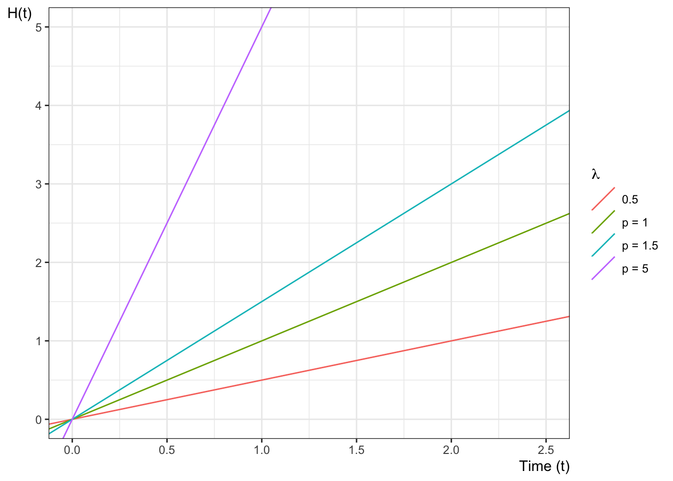
Figure 6.3 shows some examples of exponential cumulative hazard functions.

---

Figure 6.3: Examples of exponential cumulative hazard functions

6.3.6 Some Key Mathematical Relationships among Survival Concepts

Diagram:

\[ h(t) \xrightarrow[]{\int_{u=0}^t h(u)du} H(t) \xrightarrow[]{\text{exp}\left\{-H(t)\right\}} S(t) \xrightarrow[]{1-S(t)} F(t) \]

\[ h(t) \xleftarrow[\frac{\partial}{\partial t}H(t)]{} H(t) \xleftarrow[-\text{log}\left\{S(t)\right\}]{} S(t) \xleftarrow[1-F(t)]{} F(t) \]

---

Identities:

\[ \begin{aligned} S(t) &= 1 - F(t)\\ &= \text{exp}\left\{-H(t)\right\}\\ S'(t) &= -f(t)\\ H(t) &= -\text{log}\left\{S(t)\right\}\\ H'(t) &= h(t)\\ h(t) &= \frac{f(t)}{S(t)}\\ &= -\frac{\partial}{\partial t}\text{log}\left\{S(t)\right\} \\ f(t) &= h(t)\cdot S(t)\\ \end{aligned} \]

---

Some proofs (others left as exercises):

\[ \begin{aligned} S'(t) &= \frac{\partial}{\partial t}(1-F(t))\\ &= -F'(t)\\ &= -f(t)\\ \end{aligned} \]

---

\[ \begin{aligned} \frac{\partial}{\partial t}\text{log}\left\{S(t)\right\} &= \frac{S'(t)}{S(t)}\\ &= -\frac{f(t)}{S(t)}\\ &= -h(t)\\ \end{aligned} \]

---

\[ \begin{aligned} H(t) &\stackrel{\text{def}}{=}\int_{u=0}^t h(u) du\\ &= \int_0^t -\frac{\partial}{\partial u}\text{log}\left\{S(u)\right\} du\\ &= \left[-\text{log}\left\{S(u)\right\}\right]_{u=0}^{u=t}\\ &= \left[\text{log}\left\{S(u)\right\}\right]_{u=t}^{u=0}\\ &= \text{log}\left\{S(0)\right\} - \text{log}\left\{S(t)\right\}\\ &= \text{log}\left\{1\right\} - \text{log}\left\{S(t)\right\}\\ &= 0 - \text{log}\left\{S(t)\right\}\\ &=-\text{log}\left\{S(t)\right\} \end{aligned} \]

---

Corollary:

\[S(t) = \text{exp}\left\{-H(t)\right\}\]

---

Example: Time to death the US in 2004

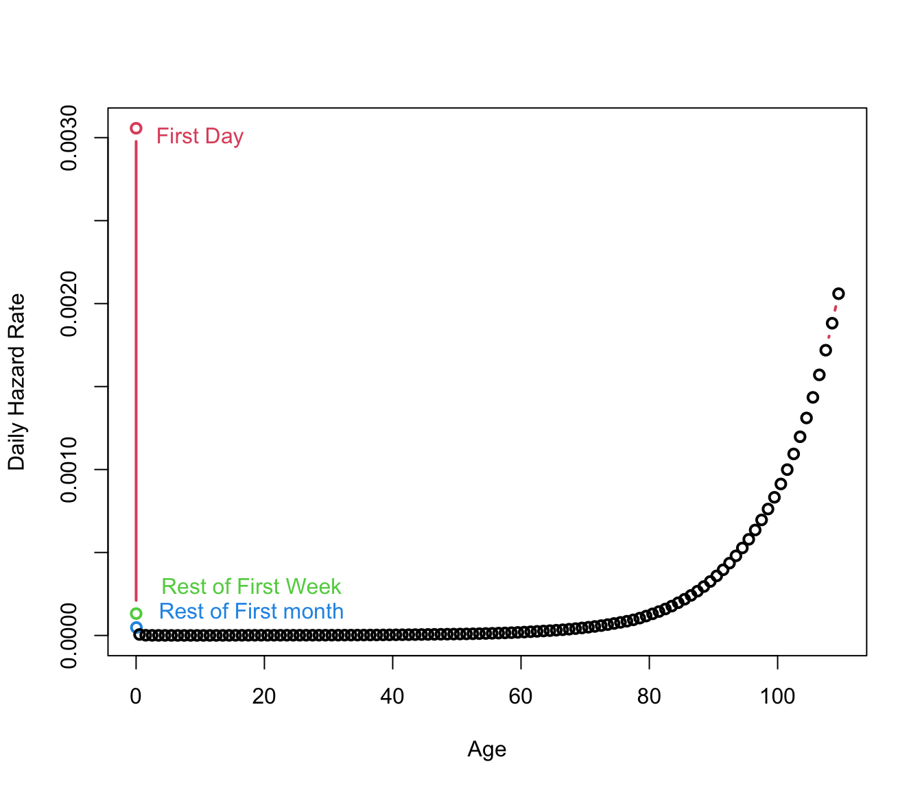
The first day is the most dangerous:

# download `survexp.rda` from: 
# paste0(
# "https://github.com/therneau/survival/raw/",
# "f3ac93704949ff26e07720b56f2b18ffa8066470/",
# "data/survexp.rda")

#(newer versions of `survival` don't have the first-year breakdown; see:
# https://cran.r-project.org/web/packages/survival/news.html)

fs::path(
  here::here(),
  "data",
  "survexp.rda") |>
  load()
s1 <- survexp.us[,"female","2004"]
age1 <- c(
  0.5/365.25,
  4/365.25,
  17.5/365.25,
  196.6/365.25,
  1:109+0.5)
s2 <- 365.25*s1[5:113]
s2 <- c(s1[1], 6*s1[2], 22*s1[3], 337.25*s1[4], s2)
cols <- rep(1,113)
cols[1] <- 2
cols[2] <- 3
cols[3] <- 4

plot(age1,s1,type="b",lwd=2,xlab="Age",ylab="Daily Hazard Rate",col=cols)

text(10,.003,"First Day",col=2)
text(18,.00030,"Rest of First Week",col=3)
text(18,.00015,"Rest of First month",col=4)

Figure 6.4: Daily Hazard Rates in 2004 for US Females

---

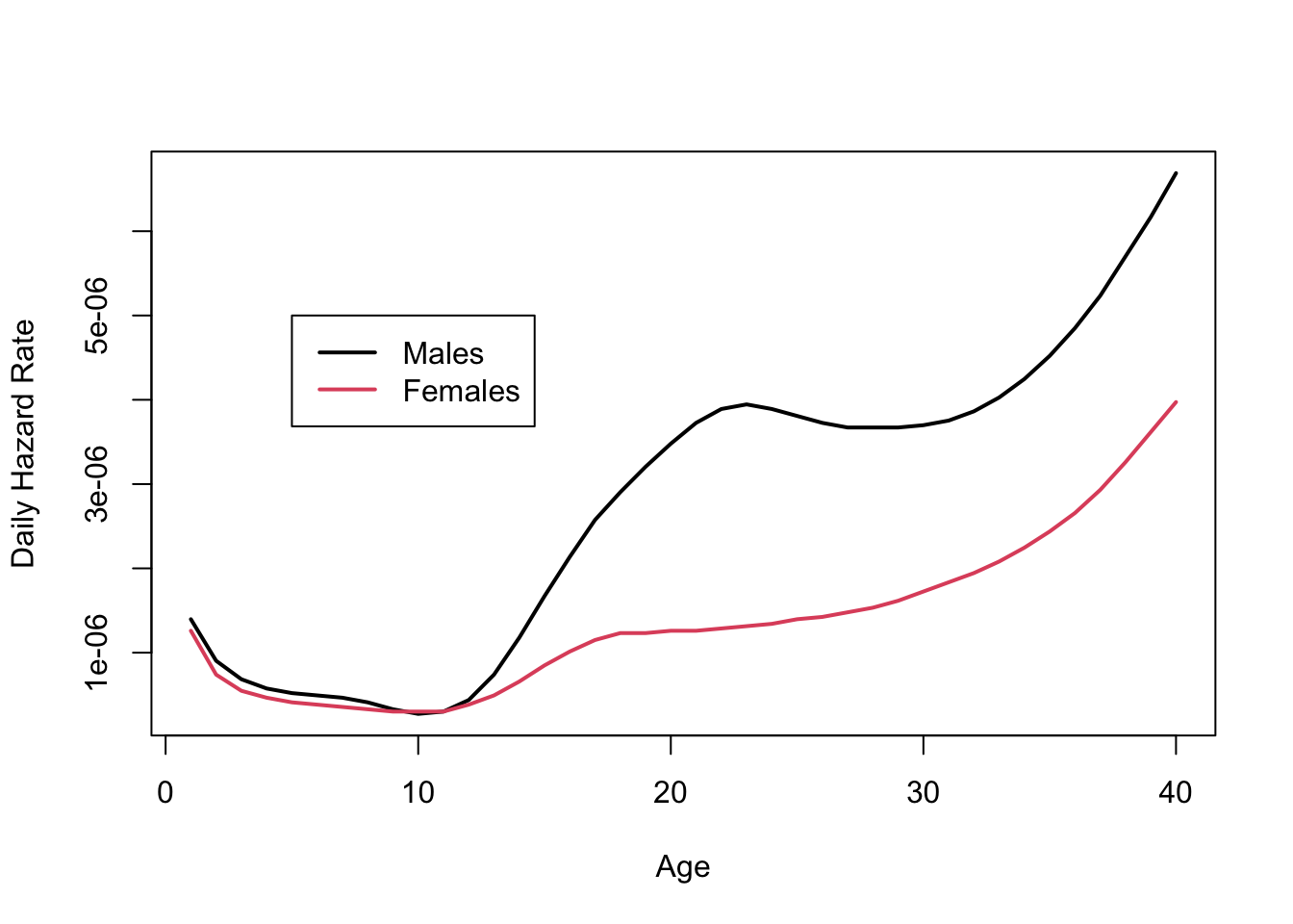
Exercise 6.1 Hypothesize why the male and female hazard functions in Figure 6.5 differ where they do?

yrs=1:40
s1 <- survexp.us[5:113,"male","2004"]
s2 <- survexp.us[5:113,"female","2004"]

age1 <- 1:109

plot(age1[yrs],s1[yrs],type="l",lwd=2,xlab="Age",ylab="Daily Hazard Rate")
lines(age1[yrs],s2[yrs],col=2,lwd=2)
legend(5,5e-6,c("Males","Females"),col=1:2,lwd=2)

Figure 6.5: Daily Hazard Rates in 2004 for US Males and Females 1-40

---

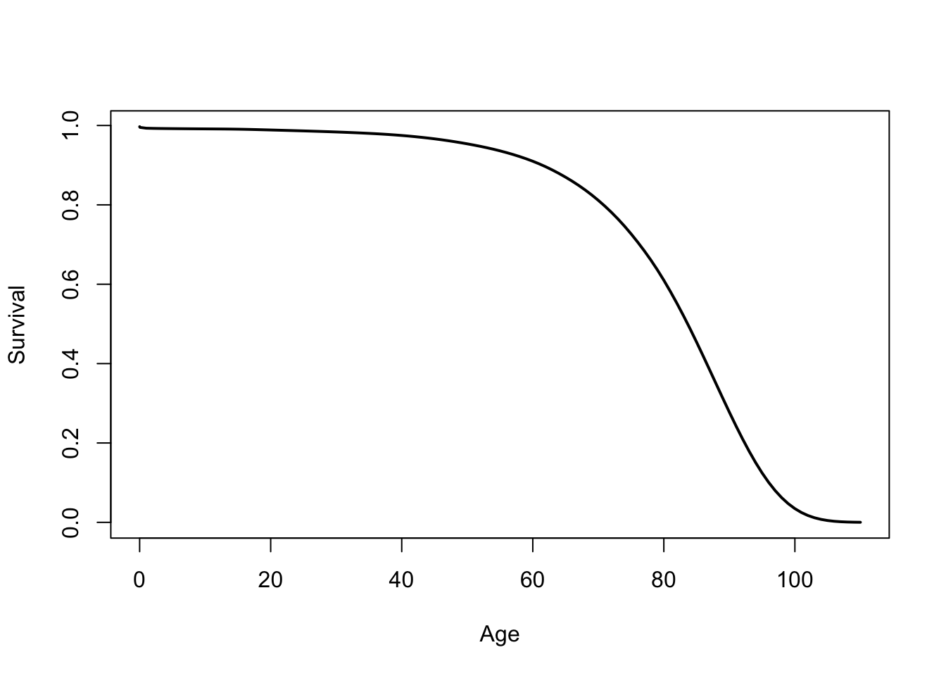
Exercise 6.2 Compare and contrast Figure 6.6 with Figure 6.4.

---

s1 <- survexp.us[,"female","2004"]

s2 <- 365.25*s1[5:113]
s2 <- c(s1[1], 6*s1[2], 21*s1[3], 337.25*s1[4], s2)
cs2 <- cumsum(s2)
age2 <- c(1/365.25, 7/365.25, 28/365.25, 1:110)
plot(age2,exp(-cs2),type="l",lwd=2,xlab="Age",ylab="Survival")

Figure 6.6: Survival Curve in 2004 for US Females

---

6.3.7 Likelihood with censoring

If an event time \(T\) is observed exactly as \(T=t\), then the likelihood of that observation is just its probability density function:

\[ \begin{aligned} \mathcal L(t) &= p(T=t)\\ &\stackrel{\text{def}}{=}f_T(t)\\ &= h_T(t)S_T(t)\\ \ell(t) &\stackrel{\text{def}}{=}\text{log}\left\{\mathcal L(t)\right\}\\ &= \text{log}\left\{h_T(t)S_T(t)\right\}\\ &= \text{log}\left\{h_T(t)\right\} + \text{log}\left\{S_T(t)\right\}\\ &= \text{log}\left\{h_T(t)\right\} - H_T(t)\\ \end{aligned} \]

---

If instead the event time \(T\) is censored and only known to be after time \(y\), then the likelihood of that censored observation is instead the survival function evaluated at the censoring time:

\[ \begin{aligned} \mathcal L(y) &=p_T(T>y)\\ &\stackrel{\text{def}}{=}S_T(y)\\ \ell(y) &\stackrel{\text{def}}{=}\text{log}\left\{\mathcal L(y)\right\}\\ &=\text{log}\left\{S(y)\right\}\\ &=-H(y)\\ \end{aligned} \]

---

What’s written above is incomplete. We also observed whether or not the observation was censored. Let \(C\) denote the time when censoring would occur (if the event did not occur first); let \(f_C(y)\) and \(S_C(y)\) be the corresponding density and survival functions for the censoring event.

Let \(Y\) denote the time when observation ended (either by censoring or by the event of interest occurring), and let \(D\) be an indicator variable for the event occurring at \(Y\) (so \(D=0\) represents a censored observation and \(D=1\) represents an uncensored observation). In other words, let \(Y \stackrel{\text{def}}{=}\min(T,C)\) and \(D \stackrel{\text{def}}{=}\mathbb 1{\{T<=C\}}\).

Then the complete likelihood of the observed data \((Y,D)\) is:

\[ \begin{aligned} \mathcal L(y,d) &= p(Y=y, D=d)\\ &= \left[p(T=y,C> y)\right]^d \cdot \left[p(T>y,C=y)\right]^{1-d}\\ \end{aligned} \]

---

Typically, survival analyses assume that \(C\) and \(T\) are mutually independent; this assumption is called “non-informative” censoring.

Then the joint likelihood \(p(Y,D)\) factors into the product \(p(Y), p(D)\), and the likelihood reduces to:

\[ \begin{aligned} \mathcal L(y,d) &= \left[p(T=y,C> y)\right]^d\cdot \left[p(T>y,C=y)\right]^{1-d}\\ &= \left[p(T=y)p(C> y)\right]^d\cdot \left[p(T>y)p(C=y)\right]^{1-d}\\ &= \left[f_T(y)S_C(y)\right]^d\cdot \left[S(y)f_C(y)\right]^{1-d}\\ &= \left[f_T(y)^d S_C(y)^d\right]\cdot \left[S_T(y)^{1-d}f_C(y)^{1-d}\right]\\ &= \left(f_T(y)^d \cdot S_T(y)^{1-d}\right)\cdot \left(f_C(y)^{1-d} \cdot S_C(y)^{d}\right) \end{aligned} \]

---

The corresponding log-likelihood is:

\[ \begin{aligned} \ell(y,d) &= \text{log}\left\{\mathcal L(y,d) \right\}\\ &= \text{log}\left\{ \left(f_T(y)^d \cdot S_T(y)^{1-d}\right)\cdot \left(f_C(y)^{1-d} \cdot S_C(y)^{d}\right) \right\}\\ &= \text{log}\left\{ f_T(y)^d \cdot S_T(y)^{1-d} \right\} + \text{log}\left\{ f_C(y)^{1-d} \cdot S_C(y)^{d} \right\}\\ \end{aligned} \] Let

• \(\theta_T\) represent the parameters of \(p_T(t)\),
• \(\theta_C\) represent the parameters of \(p_C(c)\),
• \(\theta = (\theta_T, \theta_C)\) be the combined vector of all parameters.

---

The corresponding score function is:

\[ \begin{aligned} \ell'(y,d) &= \frac{\partial}{\partial \theta} \left[ \text{log}\left\{ f_T(y)^d \cdot S_T(y)^{1-d} \right\} + \text{log}\left\{ f_C(y)^{1-d} \cdot S_C(y)^{d} \right\} \right]\\ &= \left( \frac{\partial}{\partial \theta} \text{log}\left\{ f_T(y)^d \cdot S_T(y)^{1-d} \right\} \right) + \left( \frac{\partial}{\partial \theta} \text{log}\left\{ f_C(y)^{1-d} \cdot S_C(y)^{d} \right\} \right)\\ \end{aligned} \]

---

As long as \(\theta_C\) and \(\theta_T\) don’t share any parameters, then if censoring is non-informative, the partial derivative with respect to \(\theta_T\) is:

\[ \begin{aligned} \ell'_{\theta_T}(y,d) &\stackrel{\text{def}}{=}\frac{\partial}{\partial \theta_T}\ell(y,d)\\ &= \left( \frac{\partial}{\partial \theta_T} \text{log}\left\{ f_T(y)^d \cdot S_T(y)^{1-d} \right\} \right) + \left( \frac{\partial}{\partial \theta_T} \text{log}\left\{ f_C(y)^{1-d} \cdot S_C(y)^{d} \right\} \right)\\ &= \left( \frac{\partial}{\partial \theta_T} \text{log}\left\{ f_T(y)^d \cdot S_T(y)^{1-d} \right\} \right) + 0\\ &= \frac{\partial}{\partial \theta_T} \text{log}\left\{ f_T(y)^d \cdot S_T(y)^{1-d} \right\}\\ \end{aligned} \]

---

Thus, the MLE for \(\theta_T\) won’t depend on \(\theta_C\), and we can ignore the distribution of \(C\) when estimating the parameters of \(f_T(t)=p(T=t)\).

Then:

\[ \begin{aligned} \mathcal L(y,d) &= f_T(y)^d \cdot S_T(y)^{1-d}\\ &= \left(h_T(y)^d S_T(y)^d\right) \cdot S_T(y)^{1-d}\\ &= h_T(y)^d \cdot S_T(y)^d \cdot S_T(y)^{1-d}\\ &= h_T(y)^d \cdot S_T(y)\\ &= S_T(y) \cdot h_T(y)^d \\ \end{aligned} \]

That is, if the event occurred at time \(y\) (i.e., if \(d=1\)), then the likelihood of \((Y,D) = (y,d)\) is equal to the hazard function at \(y\) times the survival function at \(y\). Otherwise, the likelihood is equal to just the survival function at \(y\).

---

The corresponding log-likelihood is:

\[ \begin{aligned} \ell(y,d) &=\text{log}\left\{\mathcal L(y,d)\right\}\\ &= \text{log}\left\{S_T(y) \cdot h_T(y)^d\right\}\\ &= \text{log}\left\{S_T(y)\right\} + \text{log}\left\{h_T(y)^d\right\}\\ &= \text{log}\left\{S_T(y)\right\} + d\cdot \text{log}\left\{h_T(y)\right\}\\ &= -H_T(y) + d\cdot \text{log}\left\{h_T(y)\right\}\\ \end{aligned} \]

In other words, the log-likelihood contribution from a single observation \((Y,D) = (y,d)\) is equal to the negative cumulative hazard at \(y\), plus the log of the hazard at \(y\) if the event occurred at time \(y\).

6.4 Parametric Models for Time-to-Event Outcomes

6.4.1 Exponential Distribution

• The exponential distribution is the base distribution for survival analysis.
• The distribution has a constant hazard \(\lambda\)
• The mean survival time is \(\lambda^{-1}\)

---

Mathematical details of exponential distribution

\[ \begin{aligned} f(t) &= \lambda \text{e}^{-\lambda t}\\ E(t) &= \lambda^{-1}\\ Var(t) &= \lambda^{-2}\\ F(t) &= 1-\text{e}^{-\lambda x}\\ S(t)&= \text{e}^{-\lambda x}\\ \ln(S(t))&=-\lambda x\\ h(t) &= -\frac{f(t)}{S(t)} = -\frac{\lambda \text{e}^{-\lambda t}}{\text{e}^{-\lambda t}}=\lambda \end{aligned} \]

---

Estimating \(\lambda\)

• Suppose we have \(m\) exponential survival times of \(t_1, t_2,\ldots,t_m\) and \(k\) right-censored values at \(u_1,u_2,\ldots,u_k\).

• A survival time of \(t_i=10\) means that subject \(i\) died at time 10. A right-censored time \(u_i=10\) means that at time 10, subject \(i\) was still alive and that we have no further follow-up.

• For the moment we will assume that the survival distribution is exponential and that all the subjects have the same parameter \(\lambda\).

We have \(m\) exponential survival times of \(t_1, t_2,\ldots,t_m\) and \(k\) right-censored values at \(u_1,u_2,\ldots,u_k\). The log-likelihood of an observed survival time \(t_i\) is \[ \text{log}\left\{\lambda \text{e}^{-\lambda t_i}\right\} = \text{log}\left\{\lambda\right\}-\lambda t_i \] and the likelihood of a censored value is the probability of that outcome (survival greater than \(u_j\)) so the log-likelihood is

\[ \begin{aligned} \ell_j(\lambda) &= \text{log}\left\{\lambda \text{e}^{u_j}\right\} \\ &= -\lambda u_j \end{aligned} \]

---

Theorem 6.6 Let \(T=\sum t_i\) and \(U=\sum u_j\). Then:

\[ \hat{\lambda}_{ML} = \frac{m}{T+U} \tag{6.3}\]

---

Proof. \[ \begin{aligned} \ell(\lambda) &= \sum_{i=1}^m( \ln \lambda-\lambda t_i) + \sum_{j=1}^k (-\lambda u_j)\\ &= m \ln \lambda -(T+U)\lambda\\ \ell'(\lambda) &=m\lambda^{-1} -(T+U)\\ \hat{\lambda} &= \frac{m}{T+U} \end{aligned} \]

---

\[ \begin{aligned} \ell''&=-m/\lambda^2\\ &< 0\\ \hat E[T] &= \hat\lambda^{-1}\\ &= \frac{T+U}{m} \end{aligned} \]

---

Fisher Information and Standard Error

\[ \begin{aligned} E[-\ell''] & = m/\lambda^2\\ \text{Var}\left(\hat\lambda\right) &\approx \left(E[-\ell'']\right)^{-1}\\ &=\lambda^2/m\\ \text{SE}\left(\hat\lambda\right) &= \sqrt{\text{Var}\left(\hat\lambda\right)}\\ &\approx \lambda/\sqrt{m} \end{aligned} \]

\(\hat\lambda\) depends on the censoring times of the censored observations, but \(\text{Var}\left(\hat\lambda\right)\) only depends on the number of uncensored observations, \(m\), and not on the number of censored observations (\(k\)).

---

6.4.2 Other Parametric Survival Distributions

• Any density on \([0,\infty)\) can be a survival distribution, but the most useful ones are all skew right.
• The most frequently used generalization of the exponential is the Weibull.
• Other common choices are the gamma, log-normal, log-logistic, Gompertz, inverse Gaussian, and Pareto.
• Most of what we do going forward is non-parametric or semi-parametric, but sometimes these parametric distributions provide a useful approach.

6.5 Nonparametric Survival Analysis

6.5.1 Basic ideas

• Mostly, we work without a parametric model.

• The first task is to estimate a survival function from data listing survival times, and censoring times for censored data.

• For example one patient may have relapsed at 10 months. Another might have been followed for 32 months without a relapse having occurred (censored).

• The minimum information we need for each patient is a time and a censoring variable which is 1 if the event occurred at the indicated time and 0 if this is a censoring time.

6.6 Example: clinical trial for pediatric acute leukemia

6.6.1 Overview of study

This is from a clinical trial in 1963 for 6-MP treatment vs. placebo for Acute Leukemia in 42 children.

• Pairs of children:

  • matched by remission status at the time of treatment (remstat: 1 = partial, 2 = complete)
  • randomized to 6-MP (exit times in t2) or placebo (exit times in t1)

• Followed until relapse or end of study.

• All of the placebo group relapsed, but some of the 6-MP group were censored (which means they were still in remission); indicated by relapse variable (0 = censored, 1 = relapse).

• 6-MP = 6-Mercaptopurine (Purinethol) is an anti-cancer (“antineoplastic” or “cytotoxic”) chemotherapy drug used currently for Acute lymphoblastic leukemia (ALL). It is classified as an antimetabolite.

6.6.2 Study design

• Clinical trial in 1963 for 6-MP treatment vs. placebo for Acute Leukemia in 42 children.
• Pairs of children:
  • matched by remission status at the time of treatment (remstat)
    • remstat = 1: partial
    • remstat = 2: complete
  • randomized to 6-MP (exit time: t2) or placebo (t1).
• Followed until relapse or end of study.
  • All of the placebo group relapsed,
  • Some of the 6-MP group were censored.

---

Table 6.1: drug6mp pediatric acute leukemia data

library(KMsurv)
data(drug6mp)
drug6mp = drug6mp |> as_tibble() |> print()
#> # A tibble: 21 × 5
#>     pair remstat    t1    t2 relapse
#>    <int>   <int> <int> <int>   <int>
#>  1     1       1     1    10       1
#>  2     2       2    22     7       1
#>  3     3       2     3    32       0
#>  4     4       2    12    23       1
#>  5     5       2     8    22       1
#>  6     6       1    17     6       1
#>  7     7       2     2    16       1
#>  8     8       2    11    34       0
#>  9     9       2     8    32       0
#> 10    10       2    12    25       0
#> # ℹ 11 more rows

6.6.3 Data documentation for drug6mp

# library(printr) # inserts help-file output into markdown output
library(KMsurv)
?drug6mp

6.6.4 Descriptive Statistics

Table 6.2: Summary statistics for drug6mp data

summary(drug6mp)
#>       pair       remstat           t1              t2          relapse     
#>  Min.   : 1   Min.   :1.00   Min.   : 1.00   Min.   : 6.0   Min.   :0.000  
#>  1st Qu.: 6   1st Qu.:2.00   1st Qu.: 4.00   1st Qu.: 9.0   1st Qu.:0.000  
#>  Median :11   Median :2.00   Median : 8.00   Median :16.0   Median :0.000  
#>  Mean   :11   Mean   :1.76   Mean   : 8.67   Mean   :17.1   Mean   :0.429  
#>  3rd Qu.:16   3rd Qu.:2.00   3rd Qu.:12.00   3rd Qu.:23.0   3rd Qu.:1.000  
#>  Max.   :21   Max.   :2.00   Max.   :23.00   Max.   :35.0   Max.   :1.000

• The average time in each group is not useful. Some of the 6-MP patients have not relapsed at the time recorded, while all of the placebo patients have relapsed.
• The median time is not really useful either because so many of the 6-MP patients have not relapsed (12/21).
• Both are biased down in the 6-MP group. Remember that lower times are worse since they indicate sooner recurrence.

6.6.5 Exponential model

• We can compute the hazard rate, assuming an exponential model: number of relapses divided by the sum of the exit times (Equation 6.3).

\[\hat\lambda = \frac{\sum_{i=1}^nD_i}{\sum_{i=1}^nY_i}\]

• For the placebo, that is just the reciprocal of the mean time:

\[ \begin{aligned} \hat \lambda_{\text{placebo}} &= \frac{\sum_{i=1}^nD_i}{\sum_{i=1}^nY_i} \\ &= \frac{\sum_{i=1}^n1}{\sum_{i=1}^nY_i} \\ &= \frac{n}{\sum_{i=1}^nY_i} \\ &= \frac{1}{\bar{Y}} \\ &= \frac{1}{8.6667} \\ &= 0.1154 \end{aligned} \]

---

• For the 6-MP group, \(\hat\lambda = 9/359 = 0.025\)

\[ \begin{aligned} \hat \lambda_{\text{6-MP}} &= \frac{\sum_{i=1}^nD_i}{\sum_{i=1}^nY_i} \\ &= \frac{9}{359} \\ &= 0.0251 \end{aligned} \]

• The estimated hazard in the placebo group is 4.6 times as large as in the 6-MP group (assuming the hazard is constant over time).

6.7 The Kaplan-Meier Product Limit Estimator

6.7.1 Estimating survival in datasets without censoring

In the drug6mp dataset, the estimated survival function for the placebo patients is easy to compute. For any time \(t\) in months, \(S(t)\) is the fraction of patients with times greater than \(t\):

6.7.2 Estimating survival in datasets with censoring

• For the 6-MP patients, we cannot ignore the censored data because we know that the time to relapse is greater than the censoring time.

• For any time \(t\) in months, we know that 6-MP patients with times greater than \(t\) have not relapsed, and those with relapse time less than \(t\) have relapsed, but we don’t know if patients with censored time less than \(t\) have relapsed or not.

• The procedure we usually use is the Kaplan-Meier product-limit estimator of the survival function.

• The Kaplan-Meier estimator is a step function (like the empirical cdf), which changes value only at the event times, not at the censoring times.

• At each event time \(t\), we compute the at-risk group size \(Y\), which is all those observations whose event time or censoring time is at least \(t\).

• If \(d\) of the observations have an event time (not a censoring time) of \(t\), then the group of survivors immediately following time \(t\) is reduced by the fraction \[\frac{Y-d}{Y}=1-\frac{d}{Y}\]

---

Definition 6.5 (Kaplan-Meier Product-Limit Estimator of Survival Function) If the event times are \(t_i\) with events per time of \(d_i\) (\(1\le i \le k\)), then the Kaplan-Meier Product-Limit Estimator of the survival function is:

\[\hat S(t) = \prod_{t_i < t} \left[\frac{1-d_i}{Y_i}\right] \tag{6.4}\]

where \(Y_i\) is the set of observations whose time (event or censored) is \(\ge t_i\), the group at risk at time \(t_i\).

---

Theorem 6.7 (Kaplan-Meier Estimate with No Censored Observations) If there are no censored data, and there are \(n\) data points, then just after (say) the third event time

\[ \begin{aligned} \hat S(t) &= \prod_{t_i < t}\left[1-\frac{d_i}{Y_i}\right] \\ &= \left[\frac{n-d_1}{n}\right] \left[\frac{n-d_1-d_2}{n-d_1}\right] \left[\frac{n-d_1-d_2-d_3}{n-d_1-d_2}\right] \\ &= \frac{n-d_1-d_2-d_3}{n} \\ &=1-\frac{d_1+d_2+d_3}{n} \\ &=1-\hat F(t) \end{aligned} \]

where \(\hat F(t)\) is the usual empirical CDF estimate.

6.7.3 Kaplan-Meier curve for drug6mp data

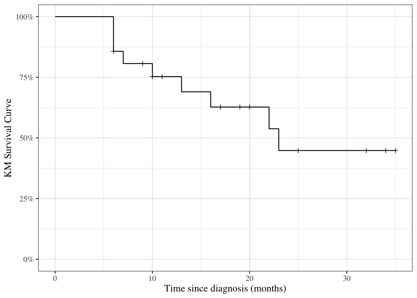
Here is the Kaplan-Meier estimated survival curve for the patients who received 6-MP in the drug6mp dataset (we will see code to produce figures like this one shortly):

# | echo: false

require(KMsurv)
data(drug6mp)
library(dplyr)
library(survival)

drug6mp_km_model1 = 
  drug6mp |> 
  mutate(surv = Surv(t2, relapse))  |> 
  survfit(formula = surv ~ 1, data = _)

library(ggfortify)
drug6mp_km_model1 |>  
  autoplot(
    mark.time = TRUE,
    conf.int = FALSE) +
  expand_limits(y = 0) +
  xlab('Time since diagnosis (months)') +
  ylab("KM Survival Curve")

Figure 6.7: Kaplan-Meier Survival Curve for 6-MP Patients

6.7.4 Kaplan-Meier calculations

Let’s compute these estimates and build the chart by hand:

library(KMsurv)
library(dplyr)
data(drug6mp)

drug6mp.v2 = 
  drug6mp |> 
  as_tibble() |> 
  mutate(
    remstat = remstat |> 
      case_match(
        1 ~ "partial",
        2 ~ "complete"
      ),
    # renaming to "outcome" while relabeling is just a style choice:
    outcome = relapse |> 
      case_match(
        0 ~ "censored",
        1 ~ "relapsed"
      )
  )

km.6mp =
  drug6mp.v2 |> 
  summarize(
    .by = t2,
    Relapses = sum(outcome == "relapsed"),
    Censored = sum(outcome == "censored")) |>
  # here we add a start time row, so the graph starts at time 0:
  bind_rows(
    tibble(
      t2 = 0, 
      Relapses = 0, 
      Censored = 0)
  ) |> 
  # sort in time order:
  arrange(t2) |>
  mutate(
    Exiting = Relapses + Censored,
    `Study Size` = sum(Exiting),
    Exited = cumsum(Exiting) |> dplyr::lag(default = 0),
    `At Risk` = `Study Size` - Exited,
    Hazard = Relapses / `At Risk`,
    `KM Factor` = 1 - Hazard,
    `Cumulative Hazard` = cumsum(`Hazard`),
    `KM Survival Curve` = cumprod(`KM Factor`)
  )

library(pander)  
pander(km.6mp)

t2	Relapses	Censored	Exiting	Study Size	Exited	At Risk	Hazard	KM Factor	Cumulative Hazard	KM Survival Curve
0	0	0	0	21	0	21	0	1	0	1
6	3	1	4	21	0	21	0.1429	0.8571	0.1429	0.8571
7	1	0	1	21	4	17	0.05882	0.9412	0.2017	0.8067
9	0	1	1	21	5	16	0	1	0.2017	0.8067
10	1	1	2	21	6	15	0.06667	0.9333	0.2683	0.7529
11	0	1	1	21	8	13	0	1	0.2683	0.7529
13	1	0	1	21	9	12	0.08333	0.9167	0.3517	0.6902
16	1	0	1	21	10	11	0.09091	0.9091	0.4426	0.6275
17	0	1	1	21	11	10	0	1	0.4426	0.6275
19	0	1	1	21	12	9	0	1	0.4426	0.6275
20	0	1	1	21	13	8	0	1	0.4426	0.6275
22	1	0	1	21	14	7	0.1429	0.8571	0.5854	0.5378
23	1	0	1	21	15	6	0.1667	0.8333	0.7521	0.4482
25	0	1	1	21	16	5	0	1	0.7521	0.4482
32	0	2	2	21	17	4	0	1	0.7521	0.4482
34	0	1	1	21	19	2	0	1	0.7521	0.4482
35	0	1	1	21	20	1	0	1	0.7521	0.4482

---

Summary

For the 6-MP patients at time 6 months, there are 21 patients at risk. At \(t=6\) there are 3 relapses and 1 censored observations.

The Kaplan-Meier factor is \((21-3)/21 = 0.857\). The number at risk for the next time (\(t=7\)) is \(21-3-1=17\).

At time 7 months, there are 17 patients at risk. At \(t=7\) there is 1 relapse and 0 censored observations. The Kaplan-Meier factor is \((17-1)/17 = 0.941\). The Kaplan Meier estimate is \(0.857\times0.941=0.807\). The number at risk for the next time (\(t=9\)) is \(17-1=16\).

---

Now, let’s graph this estimated survival curve using ggplot():

library(ggplot2)
conflicts_prefer(dplyr::filter)
km.6mp |> 
  ggplot(aes(x = t2, y = `KM Survival Curve`)) +
  geom_step() +
  geom_point(data = km.6mp |> filter(Censored > 0), shape = 3) +
  expand_limits(y = c(0,1), x = 0) +
  xlab('Time since diagnosis (months)') +
  ylab("KM Survival Curve") +
  scale_y_continuous(labels = scales::percent)

Figure 6.8: KM curve for 6MP patients, calculated by hand

6.8 Using the survival package in R

We don’t have to do these calculations by hand every time; the survival package and several others have functions available to automate many of these tasks (full list: https://cran.r-project.org/web/views/Survival.html).

6.8.1 The Surv function

To use the survival package, the first step is telling R how to combine the exit time and exit reason (censoring versus event) columns. The Surv() function accomplishes this task.

Example: Surv() with drug6mp data

library(survival)
drug6mp.v3 = 
  drug6mp.v2 |> 
  mutate(
    surv2 = Surv(
      time = t2,
      event = (outcome == "relapsed")))

print(drug6mp.v3)
#> # A tibble: 21 × 7
#>     pair remstat     t1    t2 relapse outcome   surv2
#>    <int> <chr>    <int> <int>   <int> <chr>    <Surv>
#>  1     1 partial      1    10       1 relapsed    10 
#>  2     2 complete    22     7       1 relapsed     7 
#>  3     3 complete     3    32       0 censored    32+
#>  4     4 complete    12    23       1 relapsed    23 
#>  5     5 complete     8    22       1 relapsed    22 
#>  6     6 partial     17     6       1 relapsed     6 
#>  7     7 complete     2    16       1 relapsed    16 
#>  8     8 complete    11    34       0 censored    34+
#>  9     9 complete     8    32       0 censored    32+
#> 10    10 complete    12    25       0 censored    25+
#> # ℹ 11 more rows

The output of Surv() is a vector of objects with class Surv. When we print this vector:

• observations where the event was observed are printed as the event time (for example, surv2 = 10 on line 1)

• observations where the event was right-censored are printed as the censoring time with a plus sign (+; for example, surv2 = 32+ on line 3).

6.8.2 The survfit function

Once we have constructed our Surv variable, we can calculate the Kaplan-Meier estimate of the survival curve using the survfit() function.

Note

The documentation for ?survfit isn’t too helpful; the survfit.formula documentation is better.

---

Example: survfit() with drug6mp data

Here we use survfit() to create a survfit object, which contains the Kaplan-Meier estimate:

drug6mp.km_model = survfit(
  formula = surv2 ~ 1, 
  data = drug6mp.v3)

print.survfit() just gives some summary statistics:

print(drug6mp.km_model)
#> Call: survfit(formula = surv2 ~ 1, data = drug6mp.v3)
#> 
#>       n events median 0.95LCL 0.95UCL
#> [1,] 21      9     23      16      NA

summary.survfit() shows us the underlying Kaplan-Meier table:

summary(drug6mp.km_model)
#> Call: survfit(formula = surv2 ~ 1, data = drug6mp.v3)
#> 
#>  time n.risk n.event survival std.err lower 95% CI upper 95% CI
#>     6     21       3    0.857  0.0764        0.720        1.000
#>     7     17       1    0.807  0.0869        0.653        0.996
#>    10     15       1    0.753  0.0963        0.586        0.968
#>    13     12       1    0.690  0.1068        0.510        0.935
#>    16     11       1    0.627  0.1141        0.439        0.896
#>    22      7       1    0.538  0.1282        0.337        0.858
#>    23      6       1    0.448  0.1346        0.249        0.807

---

We can specify which time points we want using the times argument:

summary(
  drug6mp.km_model, 
  times = c(0, drug6mp.v3$t2))
#> Call: survfit(formula = surv2 ~ 1, data = drug6mp.v3)
#> 
#>  time n.risk n.event survival std.err lower 95% CI upper 95% CI
#>     0     21       0    1.000  0.0000        1.000        1.000
#>    10     15       1    0.753  0.0963        0.586        0.968
#>     7     17       1    0.807  0.0869        0.653        0.996
#>    32      4       0    0.448  0.1346        0.249        0.807
#>    23      6       1    0.448  0.1346        0.249        0.807
#>    22      7       1    0.538  0.1282        0.337        0.858
#>     6     21       3    0.857  0.0764        0.720        1.000
#>    16     11       1    0.627  0.1141        0.439        0.896
#>    34      2       0    0.448  0.1346        0.249        0.807
#>    32      4       0    0.448  0.1346        0.249        0.807
#>    25      5       0    0.448  0.1346        0.249        0.807
#>    11     13       0    0.753  0.0963        0.586        0.968
#>    20      8       0    0.627  0.1141        0.439        0.896
#>    19      9       0    0.627  0.1141        0.439        0.896
#>     6     21       3    0.857  0.0764        0.720        1.000
#>    17     10       0    0.627  0.1141        0.439        0.896
#>    35      1       0    0.448  0.1346        0.249        0.807
#>     6     21       3    0.857  0.0764        0.720        1.000
#>    13     12       1    0.690  0.1068        0.510        0.935
#>     9     16       0    0.807  0.0869        0.653        0.996
#>     6     21       3    0.857  0.0764        0.720        1.000
#>    10     15       1    0.753  0.0963        0.586        0.968

---

?summary.survfit

6.8.3 Plotting estimated survival functions

We can plot survfit objects with plot(), autoplot(), or ggsurvplot():

library(ggfortify)
autoplot(drug6mp.km_model)

Kaplan-Meier Survival Curve for 6-MP Patients

# not shown:
# plot(drug6mp.km_model)

# library(survminer)
# ggsurvplot(drug6mp.km_model)

---

quantiles of survival curve

We can extract quantiles with quantile():

drug6mp.km_model |> 
  quantile(p = c(.25, .5)) |> 
  as_tibble() |> 
  mutate(p = c(.25, .5)) |> 
  relocate(p, .before = everything())

6.9 Two-sample “log-rank”/“Mantel-Haenszel” test

6.9.1 The survdiff function

?survdiff

6.9.2 Example: survdiff() with drug6mp data

Now we are going to compare the placebo and 6-MP data. We need to reshape the data to make it usable with the standard survival workflow:

library(survival)
library(tidyr)
drug6mp.v4 = 
  drug6mp.v3 |>
  select(pair, remstat, t1, t2, outcome) |> 
  # here we are going to change the data from a wide format to long:
  pivot_longer(
    cols = c(t1, t2),
    names_to = "treatment",
    values_to = "exit_time") |> 
  mutate(
    treatment = treatment |> 
      case_match(
        "t1" ~ "placebo",
        "t2" ~ "6-MP"
      ),
    outcome = if_else(
      treatment == "placebo",
      "relapsed",
      outcome
    ),
    surv = Surv(
      time = exit_time,
      event = (outcome == "relapsed"))
  )

---

Using this long data format, we can fit a Kaplan-Meier curve for each treatment group simultaneously:

drug6mp.km_model2 = 
   survfit(
  formula = surv ~ treatment, 
  data = drug6mp.v4)

---

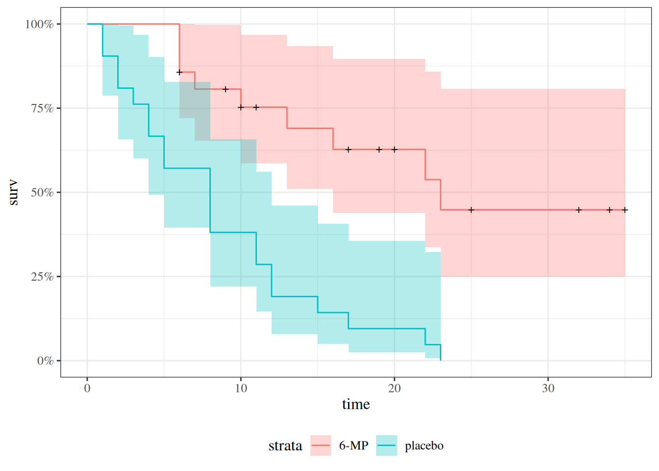
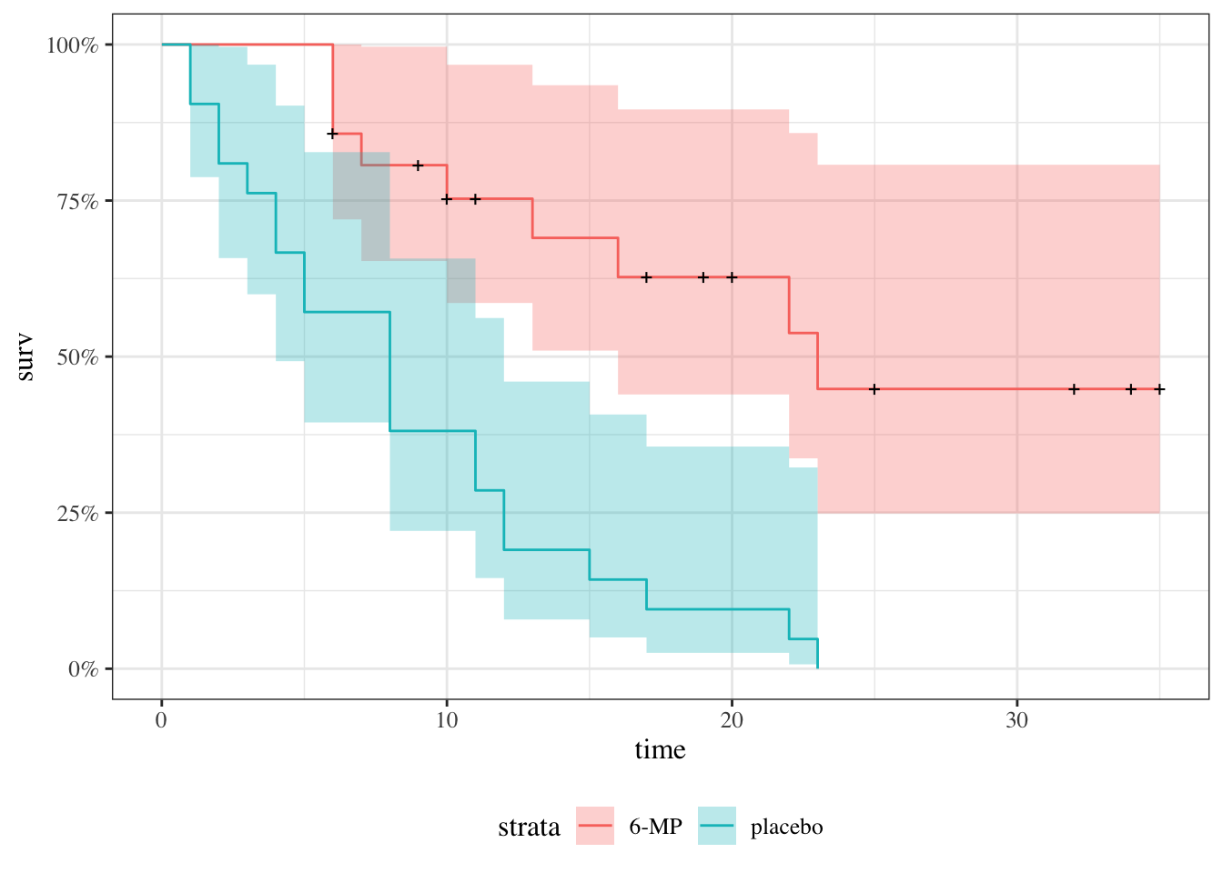
We can plot the curves in the same graph:

drug6mp.km_model2 |> autoplot()

---

We can also perform something like a t-test, where the null hypothesis is that the curves are the same:

survdiff(
  formula = surv ~ treatment,
  data = drug6mp.v4)
#> Call:
#> survdiff(formula = surv ~ treatment, data = drug6mp.v4)
#> 
#>                    N Observed Expected (O-E)^2/E (O-E)^2/V
#> treatment=6-MP    21        9     19.3      5.46      16.8
#> treatment=placebo 21       21     10.7      9.77      16.8
#> 
#>  Chisq= 16.8  on 1 degrees of freedom, p= 4e-05

By default, survdiff() ignores any pairing, but we can use strata() to perform something similar to a paired t-test:

survdiff(
  formula = surv ~ treatment + strata(pair),
  data = drug6mp.v4)
#> Call:
#> survdiff(formula = surv ~ treatment + strata(pair), data = drug6mp.v4)
#> 
#>                    N Observed Expected (O-E)^2/E (O-E)^2/V
#> treatment=6-MP    21        9     16.5      3.41      10.7
#> treatment=placebo 21       21     13.5      4.17      10.7
#> 
#>  Chisq= 10.7  on 1 degrees of freedom, p= 0.001

Interestingly, accounting for pairing reduces the significant of the difference.

6.10 Example: Bone Marrow Transplant Data

Data from Copelan et al. (1991)

---

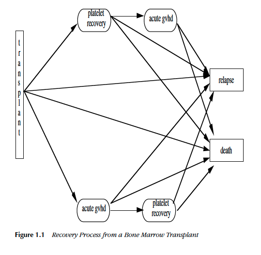
Figure 6.9: Recovery process from a bone marrow transplant (Fig. 1.1 from Klein and Moeschberger (2003))

---

6.10.1 Study design

Treatment

• allogeneic (from a donor) bone marrow transplant therapy

Inclusion criteria

• acute myeloid leukemia (AML)
• acute lymphoblastic leukemia (ALL).

Possible intermediate events

• graft vs. host disease (GVHD): an immunological rejection response to the transplant
• platelet recovery: a return of platelet count to normal levels.

One or the other, both in either order, or neither may occur.

End point events

• relapse of the disease
• death

Any or all of these events may be censored.

6.10.2 KMsurv::bmt data in R

library(KMsurv)
?bmt

6.10.3 Analysis plan

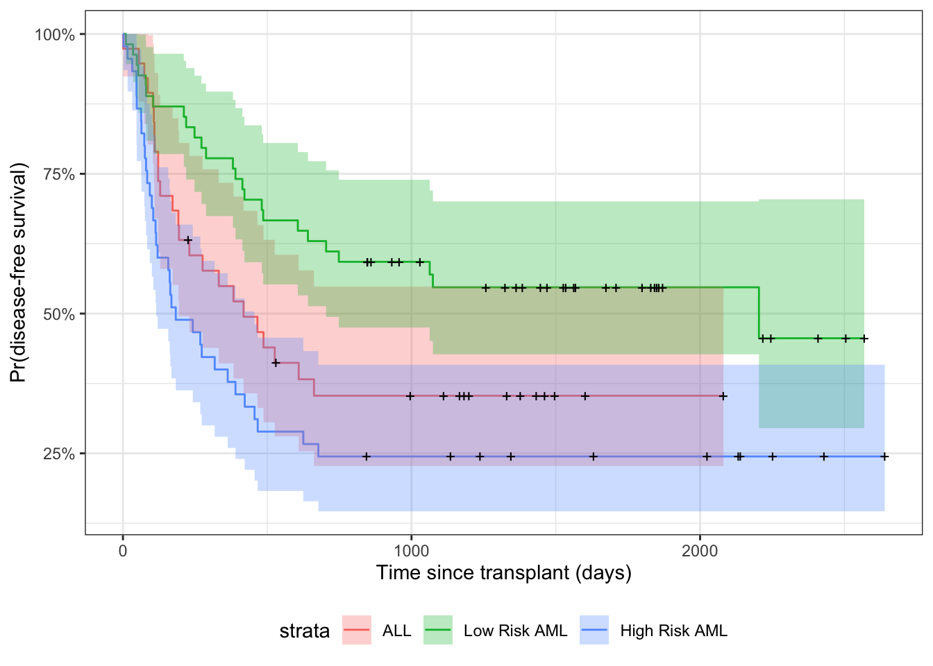
• We concentrate for now on disease-free survival (t2 and d3) for the three risk groups, ALL, AML Low Risk, and AML High Risk.
• We will construct the Kaplan-Meier survival curves, compare them, and test for differences.
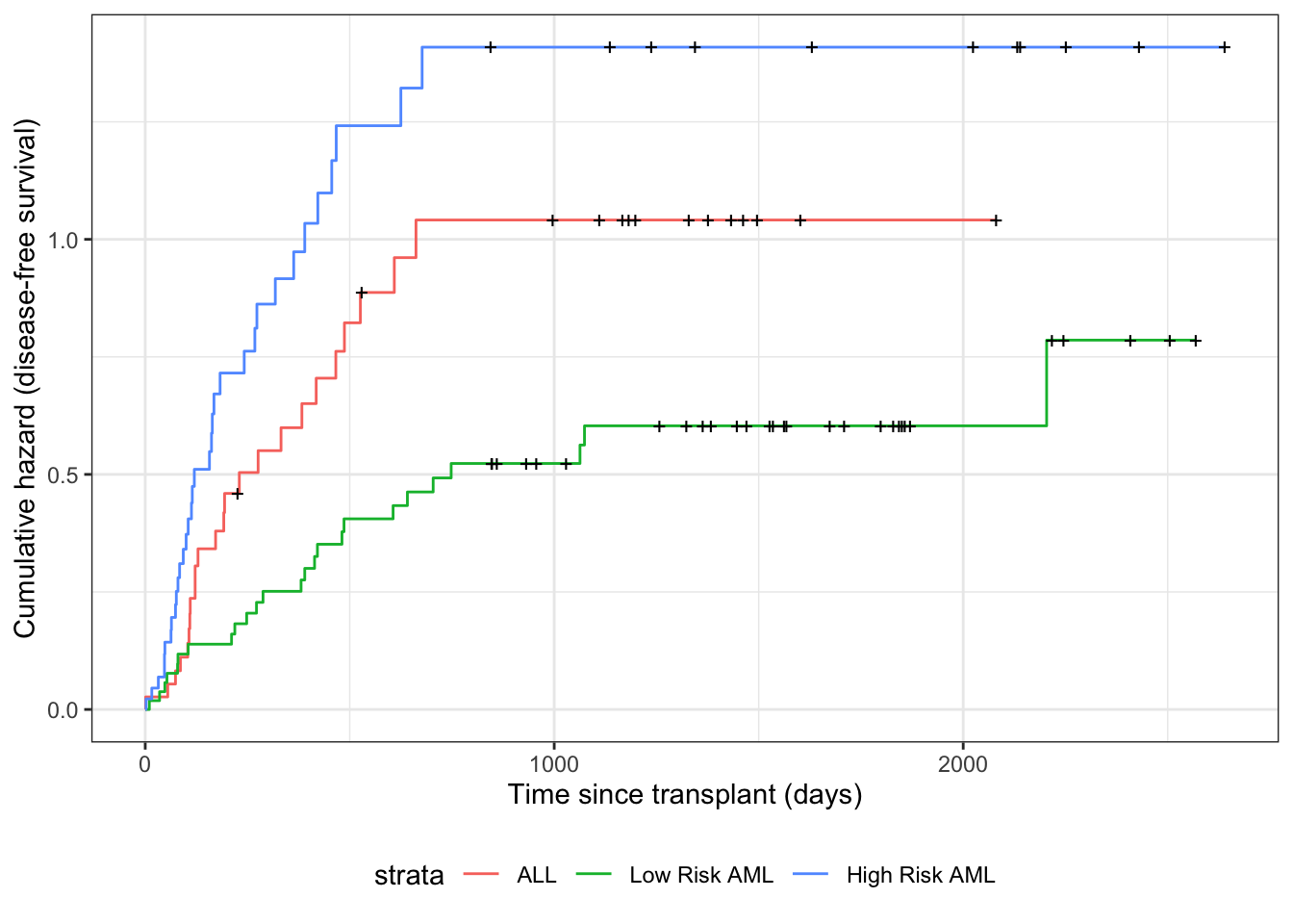
• We will construct the cumulative hazard curves and compare them.
• We will estimate the hazard functions, interpret, and compare them.

6.10.4 Survival Function Estimate and Variance

\[\hat S(t) = \prod_{t_i < t}\left[1-\frac{d_i}{Y_i}\right]\] where \(Y_i\) is the group at risk at time \(t_i\).

The estimated variance of \(\hat S(t)\) is:

Theorem 6.8 (Greenwood’s estimator for variance of Kaplan-Meier survival estimator) \[ \widehat{\text{Var}}\left(\hat S(t)\right) = \hat S(t)^2\sum_{t_i <t}\frac{d_i}{Y_i(Y_i-d_i)} \tag{6.5}\]

We can use Equation 6.5 for confidence intervals for a survival function or a difference of survival functions.

---

Kaplan-Meier survival curves

library(KMsurv)
library(survival)
data(bmt)

bmt = 
  bmt |> 
  as_tibble() |> 
  mutate(
    group = 
      group |> 
      factor(
        labels = c("ALL","Low Risk AML","High Risk AML")),
    surv = Surv(t2,d3))

km_model1 = survfit(
  formula = surv ~ group, 
  data = bmt)

library(ggfortify)
autoplot(
  km_model1, 
  conf.int = TRUE,
  ylab = "Pr(disease-free survival)",
  xlab = "Time since transplant (days)") + 
  theme_bw() +
  theme(legend.position="bottom")

Disease-Free Survival by Disease Group

---

6.10.5 Understanding Greenwood’s formula (optional)

To see where Greenwood’s formula comes from, let \(x_i = Y_i - d_i\). We approximate the solution treating each time as independent, with \(Y_i\) fixed and ignore randomness in times of failure and we treat \(x_i\) as independent binomials \(\text{Bin}(Y_i,p_i)\). Letting \(S(t)\) be the “true” survival function

\[ \begin{aligned} \hat S(t) &=\prod_{t_i<t}x_i/Y_i\\ S(t)&=\prod_{t_i<t}p_i \end{aligned} \]

\[ \begin{aligned} \frac{\hat S(t)}{S(t)} &= \prod_{t_i<t} \frac{x_i}. {p_iY_i} \\ &= \prod_{t_i<t} \frac{\hat p_i}{p_i} \\ &= \prod_{t_i<t} \left(1+\frac{\hat p_i-p_i}{p_i}\right) \\ &\approx 1+\sum_{t_i<t} \frac{\hat p_i-p_i}{p_i} \end{aligned} \]

---

\[ \begin{aligned} \text{Var}\left(\frac{\hat S(t)}{S(t)}\right) &\approx \text{Var}\left(1+\sum_{t_i<t} \frac{\hat p_i-p_i}{p_i}\right) \\ &=\sum_{t_i<t} \frac{1}{p_i^2}\frac{p_i(1-p_i)}{Y_i} \\ &= \sum_{t_i<t} \frac{(1-p_i)}{p_iY_i} \\ &\approx\sum_{t_i<t} \frac{(1-x_i/Y_i)}{x_i} \\ &=\sum_{t_i<t} \frac{Y_i-x_i}{x_iY_i} \\ &=\sum_{t_i<t} \frac{d_i}{Y_i(Y_i-d_i)} \\ \therefore\text{Var}\left(\hat S(t)\right) &\approx \hat S(t)^2\sum_{t_i<t} \frac{d_i}{Y_i(Y_i-d_i)} \end{aligned} \]

6.10.6 Test for differences among the disease groups

Here we compute a chi-square test for assocation between disease group (group) and disease-free survival:

survdiff(surv ~ group, data = bmt)
#> Call:
#> survdiff(formula = surv ~ group, data = bmt)
#> 
#>                      N Observed Expected (O-E)^2/E (O-E)^2/V
#> group=ALL           38       24     21.9     0.211     0.289
#> group=Low Risk AML  54       25     40.0     5.604    11.012
#> group=High Risk AML 45       34     21.2     7.756    10.529
#> 
#>  Chisq= 13.8  on 2 degrees of freedom, p= 0.001

6.10.7 Cumulative Hazard

\[ \begin{aligned} h(t) &\stackrel{\text{def}}{=}P(T=t|T\ge t)\\ &= \frac{p(T=t)}{P(T\ge t)}\\ &= -\frac{\partial}{\partial t}\text{log}\left\{S(t)\right\} \end{aligned} \]

The cumulative hazard (or integrated hazard) function is

\[H(t)\stackrel{\text{def}}{=}\int_0^t h(t) dt\] Since \(h(t) = -\frac{\partial}{\partial t}\text{log}\left\{S(t)\right\}\) as shown above, we have:

\[ H(t)=-\text{log}\left\{S\right\}(t) \]

---

So we can estimate \(H(t)\) as:

\[ \begin{aligned} \hat H(t) &= -\text{log}\left\{\hat S(t)\right\}\\ &= -\text{log}\left\{\prod_{t_i < t}\left[1-\frac{d_i}{Y_i}\right]\right\}\\ &= -\sum_{t_i < t}\text{log}\left\{1-\frac{d_i}{Y_i}\right\}\\ \end{aligned} \]

This is the Kaplan-Meier (product-limit) estimate of cumulative hazard.

---

Example: Cumulative Hazard Curves for Bone-Marrow Transplant (bmt) data

autoplot(
  fun = "cumhaz",
  km_model1, 
  conf.int = FALSE,
  ylab = "Cumulative hazard (disease-free survival)",
  xlab = "Time since transplant (days)") + 
  theme_bw() +
  theme(legend.position="bottom")

Figure 6.10: Disease-Free Cumulative Hazard by Disease Group

6.11 Nelson-Aalen Estimates of Cumulative Hazard and Survival

---

Definition 6.6 (Nelson-Aalen Cumulative Hazard Estimator)  

The point hazard at time \(t_i\) can be estimated by \(d_i/Y_i\), which leads to the Nelson-Aalen estimator of the cumulative hazard:

\[\hat H_{NA}(t) \stackrel{\text{def}}{=}\sum_{t_i < t}\frac{d_i}{Y_i} \tag{6.6}\]

---

Theorem 6.9 (Variance of Nelson-Aalen estimator)  

The variance of this estimator is approximately:

\[ \begin{aligned} \hat{\text{Var}}\left(\hat H_{NA} (t)\right) &= \sum_{t_i <t}\frac{(d_i/Y_i)(1-d_i/Y_i)}{Y_i}\\ &\approx \sum_{t_i <t}\frac{d_i}{Y_i^2} \end{aligned} \tag{6.7}\]

---

Since \(S(t)=\text{exp}\left\{-H(t)\right\}\), the Nelson-Aalen cumulative hazard estimate can be converted into an alternate estimate of the survival function:

\[ \begin{aligned} \hat S_{NA}(t) &= \text{exp}\left\{-\hat H_{NA}(t)\right\}\\ &= \text{exp}\left\{-\sum_{t_i < t}\frac{d_i}{Y_i}\right\}\\ &= \prod_{t_i < t}\text{exp}\left\{-\frac{d_i}{Y_i}\right\}\\ \end{aligned} \]

---

Compare these with the corresponding Kaplan-Meier estimates:

\[ \begin{aligned} \hat H_{KM}(t) &= -\sum_{t_i < t}\text{log}\left\{1-\frac{d_i}{Y_i}\right\}\\ \hat S_{KM}(t) &= \prod_{t_i < t}\left[1-\frac{d_i}{Y_i}\right] \end{aligned} \]

The product limit estimate and the Nelson-Aalen estimate often do not differ by much. The latter is considered more accurate in small samples and also directly estimates the cumulative hazard. The "fleming-harrington" method for survfit() reduces to Nelson-Aalen when the data are unweighted. We can also estimate the cumulative hazard as the negative log of the KM survival function estimate.

6.11.1 Application to bmt dataset

na_fit = survfit(
  formula = surv ~ group,
  type = "fleming-harrington",
  data = bmt)

km_fit = survfit(
  formula = surv ~ group,
  type = "kaplan-meier",
  data = bmt)

km_and_na = 
  bind_rows(
    .id = "model",
    "Kaplan-Meier" = km_fit |> fortify(surv.connect = TRUE),
    "Nelson-Aalen" = na_fit |> fortify(surv.connect = TRUE)
  ) |> 
  as_tibble()

km_and_na |> 
  ggplot(aes(x = time, y = surv, col = model)) +
  geom_step() +
  facet_grid(. ~ strata) +
  theme_bw() + 
  ylab("S(t) = P(T>=t)") +
  xlab("Survival time (t, days)") +
  theme(legend.position = "bottom")

Kaplan-Meier and Nelson-Aalen Survival Function Estimates, stratified by disease group

The Kaplan-Meier and Nelson-Aalen survival estimates are very similar for this dataset.

Copelan, Edward A, James C Biggs, James M Thompson, Pamela Crilley, Jeff Szer, John P Klein, Neena Kapoor, Belinda R Avalos, Isabel Cunningham, and Kerry Atkinson. 1991. “Treatment for Acute Myelocytic Leukemia with Allogeneic Bone Marrow Transplantation Following Preparation with BuCy2.” https://doi.org/10.1182/blood.V78.3.838.838.

Klein, John P, and Melvin L Moeschberger. 2003. Survival Analysis: Techniques for Censored and Truncated Data. Vol. 1230. Springer. https://link.springer.com/book/10.1007/b97377.