Appendix F — Introduction to Maximum Likelihood Inference

Published

Last modified: 2024-12-13: 0:43:41 (AM)


These notes are derived primarily from Dobson and Barnett (2018) (mostly chapters 1-5).

Some material was also taken from McLachlan and Krishnan (2007) and Casella and Berger (2002).


Configuring R

Functions from these packages will be used throughout this document:

Show R code
library(conflicted) # check for conflicting function definitions
# library(printr) # inserts help-file output into markdown output
library(rmarkdown) # Convert R Markdown documents into a variety of formats.
library(pander) # format tables for markdown
library(ggplot2) # graphics
library(ggeasy) # help with graphics
library(ggfortify) # help with graphics
library(dplyr) # manipulate data
library(tibble) # `tibble`s extend `data.frame`s
library(magrittr) # `%>%` and other additional piping tools
library(haven) # import Stata files
library(knitr) # format R output for markdown
library(tidyr) # Tools to help to create tidy data
library(plotly) # interactive graphics
library(dobson) # datasets from Dobson and Barnett 2018
library(parameters) # format model output tables for markdown
library(haven) # import Stata files
library(latex2exp) # use LaTeX in R code (for figures and tables)
library(fs) # filesystem path manipulations
library(survival) # survival analysis
library(survminer) # survival analysis graphics
library(KMsurv) # datasets from Klein and Moeschberger
library(parameters) # format model output tables for
library(webshot2) # convert interactive content to static for pdf
library(forcats) # functions for categorical variables ("factors")
library(stringr) # functions for dealing with strings
library(lubridate) # functions for dealing with dates and times

Here are some R settings I use in this document:

Show R code
rm(list = ls()) # delete any data that's already loaded into R

conflicts_prefer(dplyr::filter)
ggplot2::theme_set(
  ggplot2::theme_bw() + 
        # ggplot2::labs(col = "") +
    ggplot2::theme(
      legend.position = "bottom",
      text = ggplot2::element_text(size = 12, family = "serif")))

knitr::opts_chunk$set(message = FALSE)
options('digits' = 4)

panderOptions("big.mark", ",")
pander::panderOptions("table.emphasize.rownames", FALSE)
pander::panderOptions("table.split.table", Inf)
conflicts_prefer(dplyr::filter) # use the `filter()` function from dplyr() by default
legend_text_size = 9

F.1 Overview of maximum likelihood estimation

F.1.1 The likelihood function

Definition F.1 (Likelihood of a single observation) Let \(X\) be a random variable and let \(x\) be \(X\)’s observed data value. Let \(\text{p}_{\Theta}(X=x)\) be a probability model for the distribution of \(X\), with parameter vector \(\Theta\).

Then the likelihood of parameter value \(\theta\), for model \(\text{p}_{\Theta}(X=x)\) and data \(X = x\), is simply the probability of the event \(X=x\) given \(\Theta= \theta\):

\[ \begin{aligned} \mathcal{L}(\theta) &\stackrel{\text{def}}{=}\text{P}_{\theta}(X = x) \end{aligned} \]


Definition F.2 (Likelihood of a dataset) Let \(\tilde{x}\) be a dataset with corresponding random variable \(\tilde{X}\). Let \(\text{p}_{\Theta}(\tilde{X})\) be a probability model for the distribution of \(\tilde{X}\) with unknown parameter vector \(\Theta\).

Then the likelihood of parameter value \(\theta\), for model \(\text{p}_{\Theta}(X)\) and data \(\tilde{X}= \tilde{x}\), is the joint probability of \(\tilde{X}= \tilde{x}\) given \(\Theta= \theta\):

\[ \begin{aligned} \mathcal{L}(\theta) &\stackrel{\text{def}}{=}p_{\theta}(\tilde{X}= \tilde{x}) \\&=p_{\theta}(X_1=x_1, ..., X_n = x_n) \end{aligned} \]

Notation for the likelihood function

The likelihood function can be written as:

  • \(\mathcal{L}(\theta)\)
  • \(\mathcal{L}(\tilde{x};\theta)\)
  • \(\mathcal{L}(\theta; \tilde{x})\)
  • \(\mathcal{L}_{\tilde{x}}(\theta)\)
  • \(\mathcal{L}_{\theta}(\tilde{x})\)
  • \(\mathcal{L}(\tilde{x} | \theta)\)

All of these notations mean the same thing.

The likelihood is a function that takes \(\theta\) (and implicitly, \(\tilde{X}\)) as inputs and outputs a single number, the joint probability of \(\tilde{x}\) for model \(p_\Theta(\tilde{X}=\tilde{x})\) with \(\Theta = \theta\).


Theorem F.1 (Likelihood of an independent sample) For mutually independent data \(X_1, ..., X_n\):

\[\mathcal{L}(\tilde{x}|\theta) = \prod_{i=1}^n \text{p}(X_i=x_i|\theta) \tag{F.1}\]

Proof. \[ \begin{aligned} \mathcal{L}(\tilde{x}|\theta) &\stackrel{\text{def}}{=}\text{p}(X_1 = x_1, …,X_n =x_n|\theta) \\&= \prod_{i=1}^n \text{p}(X_i=x_i|\theta) \end{aligned} \] The second equality is by the definition of statistical independence.


Definition F.3 (Likelihood components) Given an \(\text{iid}\) dataset \(\tilde{x}\), the likelihood component or likelihood factor of observation \(X_i=x_i\) is the marginal likelihood of \(X_i=x_i\):

\[\mathcal{L}_i(\theta) = \text{P}(X_i=x_i)\]


Theorem F.2 For \(\text{iid}\) data \(\tilde{x}\stackrel{\text{def}}{=}x_1, \ldots, x_n\), the likelihood of the dataset is equal to the product of the observation-specific likelihood factors:

\[\mathcal{L}(\theta) = \prod_{i=1}^n\mathcal{L}_i(\theta)\]


F.1.2 The maximum likelihood estimate

Definition F.4 (Maximum likelihood estimate) The maximum likelihood estimate of a parameter vector \(\Theta\), denoted \(\hat\theta_{\text{ML}}\), is the value of \(\Theta\) that maximizes the likelihood:

\[ \hat\theta_{\text{ML}}\stackrel{\text{def}}{=}\arg \max_\Theta\mathcal{L}(\Theta) \tag{F.2}\]

F.1.3 Finding the maximum of a function

Recall from calculus: the maxima of a continuous function \(f(x)\) over a range of input values \(\mathcal{R}(x)\) can be found either:

  • at the edges of the range of input values, OR:
  • where the function is flat (i.e. where the gradient function \(f'(x) = 0\)) AND the second derivative is negative definite (\(f''(x) < 0\)).

F.1.4 Directly maximizing the likelihood function for iid data

To find the maximizer(s) of the likelihood function, we need to solve \(\mathcal{L}'(\theta) = 0\) for \(\theta\). However, even for mutually independent data, we quickly run into a problem:

\[ \begin{aligned} \mathcal{L}'(\theta) &= \frac{\partial}{\partial \theta} \mathcal{L}(\theta) \\ &= \frac{\partial}{\partial \theta} \prod_{i=1}^n p(X_i=x_i|\theta) \end{aligned} \tag{F.3}\]

The derivative of the likelihood of independent data is the derivative of a product. We will have to perform a massive application of the product rule to evaluate this derivative.

F.1.5 The log-likelihood function

It is typically easier to work with the log of the likelihood function:

Definition F.5 (Log-likelihood) The log-likelihood of parameter value \(\theta\), for model \(\text{p}_{\Theta}(\tilde{X})\) and data \(\tilde{X}= \tilde{x}\), is the natural logarithm of the likelihood1:

\[\ell(\theta) \stackrel{\text{def}}{=}\text{log}\left\{\mathcal{L}(\theta)\right\}\]


Definition F.6 (Log-likelihood components) Given a dataset \(\tilde{X}= \tilde{x}\), the log-likelihood component of observation \(X_i=x_i\) is the natural logarithm of the likelihood component:

\[\ell_i(\theta) \stackrel{\text{def}}{=}\text{log}\left\{\mathcal{L}_i(\theta)\right\}\]


Theorem F.3 The likelihood and log-likelihood have the same maximizer:

\[ \arg \max_\theta\mathcal{L}(\theta) = \arg \max_\theta\ell(\theta) \]

Proof. Left to the reader.


Theorem F.4 (Log-likelihood of an \(\text{iid}\) sample) For \(\text{iid}\) data \(X_1, ..., X_n\) with shared distribution \(\text{p}(X=x)\):

\[\ell(x|\theta) = \sum_{i=1}^n \text{log}\left\{p(X=x_i|\theta)\right\} \tag{F.4}\]

Proof. \[ \begin{aligned} \ell(x|\theta) &\stackrel{\text{def}}{=}\text{log}\left\{\mathcal{L}(\tilde{x}|\theta)\right\} \\&= \text{log}\left\{\prod_{i=1}^n \text{p}(X_i=x_i|\theta)\right\} \\&= \sum_{i=1}^n \text{log}\left\{p(X=x_i|\theta)\right\} \end{aligned} \]


For \(\text{iid}\) data, we will have a much easier time taking the derivative of the log-likelihood:

Theorem F.5 (Derivative of the log-likelihood function for \(\text{iid}\) data) For \(\text{iid}\) data:

\[\ell'(\theta) = \sum_{i=1}^n\frac{\partial}{\partial \theta} \text{log}\left\{\text{p}(X=x_i|\theta)\right\} \tag{F.5}\]

Proof. \[ \begin{aligned} \ell'(\theta) &= \frac{\partial}{\partial \theta} \ell(\theta) \\ &= \frac{\partial}{\partial \theta} \sum_{i=1}^n \text{log}\left\{\text{p}(X=x_i|\theta)\right\} \\ &= \sum_{i=1}^n \frac{\partial}{\partial \theta} \text{log}\left\{\text{p}(X=x_i|\theta)\right\} \end{aligned} \]


F.1.6 The score function

The first derivative2 of the log-likelihood, \(\ell'(\theta)\), is important enough to have its own name: the score function.

Definition F.7 (Score function) The score function of a statistical model \(\text{p}(\tilde{X}=\tilde{x})\) is the gradient (i.e., first derivative) of the log-likelihood of that model:

\[\ell'(\theta) \stackrel{\text{def}}{=}\frac{\partial}{\partial \theta} \ell(\theta)\]

We often skip writing the arguments \(x\) and/or \(\theta)\), so \(\ell' \stackrel{\text{def}}{=}\ell'(\tilde{x};\theta) \stackrel{\text{def}}{=}\ell'(\theta)\).3 Some statisticians use \(U\) or \(S\) instead of \(\ell'\). I prefer \(\ell'\). Why use up extra letters?

F.1.7 Asymptotic distribution of the maximum likelihood estimate

We learned how to quantify our uncertainty about these maximum likelihood estimates; with sufficient sample size, \(\hat\theta_{\text{ML}}\) has an approximately Gaussian distribution (Newey and McFadden 1994):

\[ \hat\theta_{ML} \dot \sim N(\theta,\mathcal I(\theta)^{-1}) \]

Recall:

  • \(\mathcal{I}(\theta) \stackrel{\text{def}}{=}\mathbb{E}\left[I(\tilde{X};\theta)\right]\)
  • \(I(\tilde{X},\theta) \stackrel{\text{def}}{=}-\ell''(\tilde{X};\theta)\)

We can estimate \(\mathcal{I}(\theta)\) using either \(\mathcal{I}(\hat\theta_{\text{ML}})\) or \(I(\tilde{x}; \hat\theta_{\text{ML}})\).

So we can estimate the standard error of \(\hat\theta_k\) as:

\[ \widehat{\text{SE}}\left(\hat\theta_k\right) = \sqrt{\left[\left(\hat{\mathcal{I}}\left(\hat\theta_{\text{ML}}\right)\right)^{-1}\right]_{kk}} \]

F.1.8 The (Fisher) (expected) information matrix

The variance of \(\ell'(x,\theta)\), \({Cov}\left\{ \ell'(x,\theta) \right\}\), is also very important; we call it the “expected information matrix”, “Fisher information matrix”, or just “information matrix”, and we represent it using the symbol \(\mathcal{I}\left(I\right)\) (\frakturI in Unicode, \mathfrak{I} in LaTeX).

\[ \begin{aligned} \mathcal{I} \stackrel{\text{def}}{=}\mathcal{I}(\theta) \\ &\stackrel{\text{def}}{=}\text{Cov}\left(\ell'|\theta\right) \\ &= \mathbb{E}[ \ell'{\ell'}^{\top} ] - \mathbb{E}[ \ell' ] \ \mathbb{E}[ \ell' ]^{\top} \end{aligned} \]

The elements of \(\mathfrak{I}\) are:

\[ \begin{aligned} \mathfrak{I}_{ij} &\stackrel{\text{def}}{=}\text{Cov}\left({\ell'}_{i},{\ell'}_{j}\right) \\ &= \mathbb{E}[ \ell_{i}'\ell_{j}' ] - \mathbb{E}[ {\ell'}_{i} ] \mathbb{E}[ {\ell'}_{j} ] \end{aligned} \]

Here,

\[ \begin{aligned} \mathbb{E}\left[\ell'\right] &\stackrel{\text{def}}{=}\int_{x \in \mathcal{R}(x)} { \ell'(x,\theta) \text{p}(X = x | \theta) dx } \\ &= \int_{x \in \mathcal{R}(X)} { \left( \frac{\partial}{\partial \theta} \text{log}\left\{\text{p}(X = x | \theta)\right\} \right) \text{p}(X = x | \theta) dx } \\ &= \int_{x \in \mathcal{R}(X)} { \frac {\frac{\partial}{\partial \theta} \text{p}(X = x | \theta)} {\text{p}(X = x | \theta)} \text{p}(X = x | \theta) dx } \\ &= \int_{x \in \mathcal{R}(X)} { \frac{\partial}{\partial \theta} \text{p}(X = x | \theta) dx } \end{aligned} \]

And similarly

\[ \mathbb{E}\left[\ell' \ell'^{\top}\right] \stackrel{\text{def}}{=} \int_{x \in R(x)} {\ell'(x,\theta)\ell'(x,\theta)^{\top}\ \text{p}\left(X = x | \theta\right)\ dx} \]

Note that \(\mathbb{E}\left[\ell'\right]\) and \(\mathbb{E}\left[\ell'{\ell'}^{\top}\right]\) are functions of \(\theta\) but not of \(x\); the expectation operator removed \(x\).

Also note that for most of the distributions you are familiar with (including Gaussian, binomial, Poisson, exponential):

\[\mathbb{E}\left[\ell'\right] = 0\]

So

\[\mathcal{I}\left(\theta\right) = \mathbb{E}\left[\ell'{\ell'}^{\top} \right]\]

Moreover, for those distributions (called the “exponential family”), we have:

\[ \mathfrak{I} = -\mathbb{E}\left[\ell''\right] = \mathbb{E}\left[- \ell''\right] \]

(see Dobson and Barnett (2018), §3.17), where

\[\ell'' \stackrel{\text{def}}{=}\frac{\partial}{\partial \theta}\ell^{'(x,\theta)^{\top}} = \frac{\partial}{\partial \theta}\frac{\partial}{\partial \theta^{\top}}\ell(x,\theta)\]

is the \(p \times p\) matrix whose elements are:

\[\ell_{ij}'' \stackrel{\text{def}}{=}\frac{\partial}{\partial \theta_{i}}\frac{\partial}{\partial \theta_{j}}\text{log}\left\{ p\left( X = x \mid \theta \right)\right\}\]

\(\ell''\) is called the “Hessian”4 of the log-likelihood function.

Sometimes, we use \(I(\theta;x) \stackrel{\text{def}}{=}- \ell''\) (note the standard-font “I” here). \(I(\theta;x)\) is the observed information, precision, or concentration matrix (Negative Hessian).

Key point

The asymptotics of MLEs gives us \({\widehat{\theta}}_{ML} \sim N\left( \theta,\mathfrak{I}^{- 1}(\theta) \right)\), approximately, for large sample sizes.

We can estimate \(\mathcal{I}^{- 1}(\theta)\) by working out \(\mathbb{E}\left[-\ell''\right]\) or \(\mathbb{E}\left[\ell'{\ell'}^{\top}\right]\) and plugging in \(\hat\theta_{\text{ML}}\), but sometimes we instead use \(I(\hat\theta_{\text{ML}},\tilde{x})\) for convenience; there are some cases where it’s provably better according to some criteria (Efron and Hinkley (1978)).

F.1.9 Iterative maximization

(c.f., Dobson and Barnett (2018), Chapter 4)

Later, when we are trying to find MLEs for likelihoods which we can’t easily differentiate, we will “hill-climb” using the Newton-Raphson algorithm:

\[ \begin{aligned} {\widehat{\theta}}^* &\leftarrow {\widehat{\theta}}^* + \left(I\left(\tilde{y};{\widehat{\theta}}^*\right)\right)^{-1} \ell'\left(\tilde{y};{\widehat{\theta}}^*\right) \\ &= {\widehat{\theta}}^* - \left(\ell''\left(\tilde{y};{\widehat{\theta}}^*\right)\right)^{-1} \ell'\left(\tilde{y};{\widehat{\theta}}^*\right) \end{aligned} \]


The reasoning for this algorithm is that we can approximate the the score function using the first-order Taylor polynomial:

\[ \begin{aligned} \ell'(\theta) &\approx \ell'^*(\theta) \\ &\stackrel{\text{def}}{=}\ell'({\widehat{\theta}}^*) + \ell''({\widehat{\theta}}^*)(\theta- {\widehat{\theta}}^*) \end{aligned} \]


The approximate score function, \(\ell'^*(\theta)\), is a linear function of \(\theta\), so it is easy to solve the corresponding approximate score equation, \(\ell'^*(\theta) = 0\), for \(\theta\):

\[ \begin{aligned} \theta &= {\widehat{\theta}}^* - \ell'({\widehat{\theta}}^*) \cdot\left(\ell''({\widehat{\theta}}^*)\right)^{-1} \end{aligned} \]


For computational simplicity, we will sometimes use \(\mathfrak{I}^{- 1}(\theta)\) in place of \(I\left( \widehat{\theta},y \right)\); doing so is called “Fisher scoring” or the “method of scoring”. Note that this is the opposite of the substitution that we are making for estimating the variance of the MLE; this time we should technically use the observed information but we use the expected information instead.


There’s also an “empirical information matrix” (see McLachlan and Krishnan (2007)):

\[I_{e}(\theta,y) \stackrel{\text{def}}{=}\sum_{i = 1}^{n}{\ell_{i}'\ {\ell_{i}'}^{\top}} - \frac{1}{n}\ell'{\ell'}^{\top}\]

where \(\ell_{i}\) is the log-likelihood of the ith observation. Note that \(\ell' = \sum_{i = 1}^{n}\ell_{i}'\).

\(\frac{1}{n}I_{e}(\theta,y)\) is the sample equivalent of

\[\mathfrak{I \stackrel{\text{def}}{=}I(}\theta) \stackrel{\text{def}}{=}{Cov}\left( \ell'|\theta \right) = E[ \ell'{\ell'}^{\top} ] - E[ \ell' ]\ E[ \ell' ]^{\top}\]

\[\left\{ \mathfrak{I}_{jk} \stackrel{\text{def}}{=}{Cov}\left( {\ell'}_{j},{\ell'}_{k} \right) = E[ \ell_{j}'\ell_{k}' ] - E[ {\ell'}_{j} ] E[ {\ell'}_{k} ] \right\}\]

\(I_{e}(\theta,y)\) is sometimes computationally easier to compute for Newton-Raphson-type maximization algorithms.

c.f. https://en.wikipedia.org/wiki/Newton%27s_method_in_optimization

F.1.10 Quantifying (un)certainty of MLEs

Confidence intervals for MLEs

An asymptotic approximation of a 95% confidence interval for \(\theta_k\) is

\[ \hat\theta_{\text{ML}}\pm z_{0.975} \times \widehat{\text{SE}}\left(\hat\theta_k\right) \]

where \(z_\beta\) the \(\beta\) quantile of the standard Gaussian distribution.

p-values and hypothesis tests for MLEs

(to add)

Likelihood ratio tests for MLEs

log(likelihood ratio) tests (c.f. Dobson and Barnett 2018, sec. 5.7):

\[-2\ell_{0} \sim \chi^{2}(p - q)\]

See also https://online.stat.psu.edu/stat504/book/export/html/657

Prediction intervals for MLEs

\[\overline{X} \in [ \widehat{\mu} \pm z_{1 - \alpha\text{/}2}\frac{\sigma}{m} ]\]

Where \(m\) is the sample size of the new data to be predicted (typically 1, except for binary outcomes, where it needs to be bigger for prediction intervals to make sense)

F.2 Example: Maximum likelihood for Tropical Cyclones in Australia

(Adapted from Dobson and Barnett (2018) §1.6.5)

F.2.1 Data

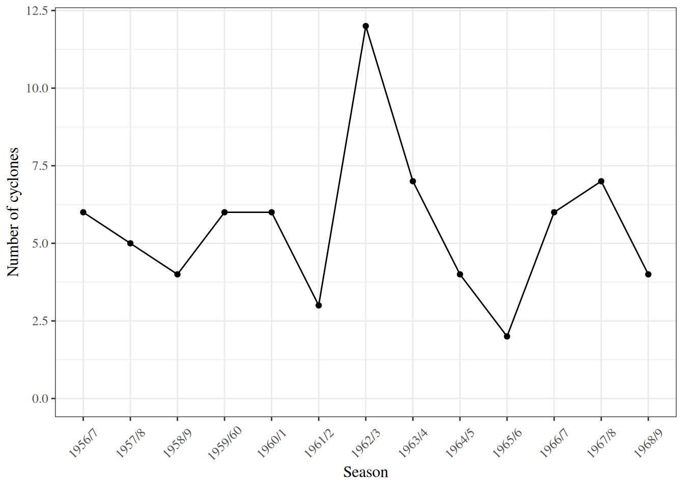
The cyclones dataset in the dobson package (Table F.1) records the number of tropical cyclones in Northeastern Australia during 13 November-to-April cyclone seasons (more details in Dobson and Barnett (2018) §1.6.5 and help(cyclones, package = "dobson")). Figure F.1 graphs the number of cyclones (y-axis) by season (x-axis). Let’s use \(Y_i\) to represent these counts, where \(i\) is an indexing variable for the seasons and \(Y_i\) is the number of cyclones in season \(i\).

F.2.2 Exploratory analysis

Suppose we want to learn about how many cyclones to expect per season.

Show R code
library(dobson)
library(dplyr)
data(cyclones)
library(pander)
pander(cyclones |> relocate(season, .before = everything()))
Table F.1: Number of tropical cyclones during a season from November to April in Northeastern Australia
season years number
1 1956/7 6
2 1957/8 5
3 1958/9 4
4 1959/60 6
5 1960/1 6
6 1961/2 3
7 1962/3 12
8 1963/4 7
9 1964/5 4
10 1965/6 2
11 1966/7 6
12 1967/8 7
13 1968/9 4
Show R code
library(ggplot2)
library(dplyr)
cyclones |>
  mutate(years = years |> factor(levels = years)) |>
  ggplot(aes(x = years, y = number, group = 1)) +
  geom_point() +
  geom_line() +
  xlab("Season") +
  ylab("Number of cyclones") +
  expand_limits(y = 0) +
  theme(axis.text.x = element_text(vjust = .5, angle = 45))
Figure F.1: Number of tropical cyclones per season in northeastern Australia, 1956-1969

There’s no obvious correlation between adjacent seasons, so let’s assume that each season is independent of the others.

Let’s also assume that they are identically distributed; let’s denote this distribution as \(P(Y=y)\) (note that there’s no index \(i\) in this expression, since we are assuming the \(Y_i\)s are identically distributed). We can visualize the distribution using a bar plot (Figure F.2). Table F.2 provides summary statistics.

Show R code
cyclones |>
  ggplot() +
  geom_histogram(aes(x = number)) +
  expand_limits(x = 0) +
  xlab("Number of cyclones") +
  ylab("Count (number of seasons)")
Figure F.2: Bar plot of cyclones per season
Show R code
n = nrow(cyclones)
sumx = cyclones |> pull(number) |> sum()
xbar =  cyclones |> pull(number) |> mean()

cyclones |> table1::table1(x = ~ number)
Table F.2: Summary statistics for cyclones data
Overall
(N=13)
number
Mean (SD) 5.54 (2.47)
Median [Min, Max] 6.00 [2.00, 12.0]

F.2.3 Model

We want to estimate \(P(Y=y)\); that is, \(P(Y=y)\) is our estimand.

We could estimate \(P(Y=y)\) for each value of \(y\) in \(0:\infty\) separately (“nonparametrically”) using the fraction of our data with \(Y_i=y\), but then we would be estimating an infinitely large set of parameters, and we would have low precision. We will probably do better with a parametric model.

Exercise F.1 What parametric probability distribution family might we use to model this empirical distribution?

Solution. Let’s use the Poisson. The Poisson distribution is appropriate for this data , because the data are counts that could theoretically take any integer value (discrete) in the range \(0:\infty\). Visually, the plot of our data closely resembles a Poisson or binomial distribution. Since cyclones do not have an “upper limit” on the number of events we could potentially observe in one season, the Poisson distribution is more appropriate than the binomial.

Exercise F.2 Write down the Poisson distribution’s probability mass function.

Solution. \[P(Y=y) = \frac{\lambda^{y} e^{-\lambda}}{y!} \tag{F.6}\]

F.2.4 Estimating the model parameters using maximum likelihood

Now, we can estimate the parameter \(\lambda\) for this distribution using maximum likelihood estimation.

What is the likelihood?

Exercise F.3 Write down the likelihood (probability mass function or probability density function) of a single observation \(x\), according to your model.

Solution. \[ \begin{aligned} \mathcal{L}(\lambda; x) &= p(X=x|\Lambda = \lambda)\\ &= \frac{\lambda^x e^{-\lambda}}{x!}\\ \end{aligned} \]

Exercise F.4 Write down the vector of parameters in your model.

Solution. There is only one parameter, \(\lambda\):

\[\theta = (\lambda)\]

Exercise F.5 Write down the population mean and variance of a single observation from your chosen probability model, as a function of the parameters (extra credit - derive them).

Solution.

  • Population mean: \(\text{E}[X]=\lambda\)
  • Population variance: \(\text{Var}(X)=\lambda\)

Exercise F.6 Write down the likelihood of the full dataset.

Solution. \[ \begin{aligned} \mathcal{L}(\lambda; \tilde{x}) &= \text{P}(\tilde{X}= \tilde{x}) \\ &= \text{P}(X_1 = x_1, X_2 = x_2, ..., X_{13} = x_{13}) \\ &= \prod_{i=1}^{13} \text{P}(X_i = x_i) \\ &= \prod_{i=1}^{13} \frac{\lambda^{x_i} e^{-\lambda}}{x_i!} \end{aligned} \]

Exercise F.7 Graph the likelihood as a function of \(\lambda\).

Solution.

Show R code
lik = function(lambda, y = cyclones$number, n = length(y)) 
{
lambda^sum(y) * exp(-n*lambda) / prod(factorial(y))
}

library(ggplot2)
lik_plot = 
ggplot() +
geom_function(fun = lik, n = 1001) +
xlim(min(cyclones$number), max(cyclones$number)) +
ylab("likelihood") +
xlab('lambda')

print(lik_plot)
Figure F.3: Likelihood of Dobson cyclone data

Exercise F.8 Write down the log-likelihood of the full dataset.

Solution. \[ \begin{aligned} \ell(\lambda; \tilde{x}) &= \text{log}\left\{\mathcal{L}(\lambda;\tilde{x})\right\}\\ &= \text{log}\left\{\prod_{i = 1}^n\frac{\lambda^{x_i}\text{e}^{-\lambda}}{x_i!}\right\}\\ &= \sum_{i = 1}^n\text{log}\left\{\frac{\lambda^{x_i}\text{e}^{-\lambda}}{x_i!}\right\}\\ &= \sum_{i = 1}^n{\text{log}\left\{\lambda^{x_i}\right\} +\text{log}\left\{\text{e}^{-\lambda}\right\} - \text{log}\left\{x_i!\right\}}\\ &= \sum_{i = 1}^n{x_i\text{log}\left\{\lambda\right\} -\lambda - \text{log}\left\{x_i!\right\}}\\ &= \sum_{i = 1}^nx_i\text{log}\left\{\lambda\right\} - \sum_{i = 1}^n\lambda - \sum_{i = 1}^n\text{log}\left\{x_i!\right\}\\ &= \sum_{i = 1}^nx_i\text{log}\left\{\lambda\right\} - n\lambda - \sum_{i = 1}^n\text{log}\left\{x_i!\right\}\\ \end{aligned} \]

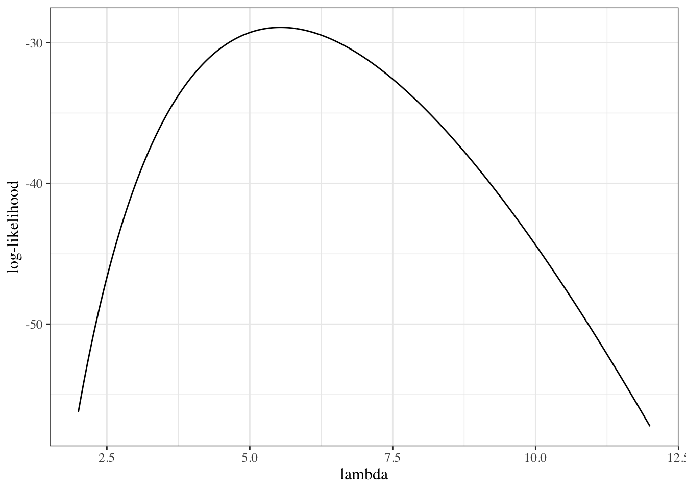
Exercise F.9 Graph the log-likelihood as a function of \(\lambda\).

Solution.

Show R code

loglik = function(lambda, y = cyclones$number, n = length(y))
{
sum(y) * log(lambda) - n*lambda - sum(log(factorial(y)))
}

ll_plot = ggplot() +
geom_function(fun = loglik, n = 1001) +
xlim(min(cyclones$number), max(cyclones$number)) +
ylab("log-likelihood") +
xlab('lambda')
ll_plot
Figure F.4: log-likelihood of Dobson cyclone data

The score function

Exercise F.10 Derive the score function for the dataset.

Solution. The score function is the first derivative of the log-likelihood:

\[ \begin{aligned} \ell'( \lambda; \tilde{x} ) &= \frac{\partial}{\partial \lambda}{\sum_{i = 1}^nx_i\text{log}\left\{\lambda\right\} - n\lambda - \sum_{i = 1}^n\text{log}\left\{x_i!\right\}}\\ &= \frac{\partial}{\partial \lambda}\sum_{i = 1}^nx_i\text{log}\left\{\lambda\right\} - \frac{\partial}{\partial \lambda}n\lambda - \frac{\partial}{\partial \lambda}\sum_{i = 1}^n\text{log}\left\{x_i!\right\}\\ &= \sum_{i = 1}^nx_i\frac{\partial}{\partial \lambda}\text{log}\left\{\lambda\right\} - n\frac{\partial}{\partial \lambda}\lambda - \sum_{i = 1}^n\frac{\partial}{\partial \lambda}\text{log}\left\{x_i!\right\}\\ &= \sum_{i = 1}^nx_i\frac{1}{\lambda} - n - 0\\ &= \frac{1}{\lambda} \sum_{i = 1}^nx_i- n \\&= \left(\frac{1}{\lambda} n \bar{x}\right) - n \\&= \left(\frac{1}{\lambda} 72\right) - 13 \end{aligned} \]

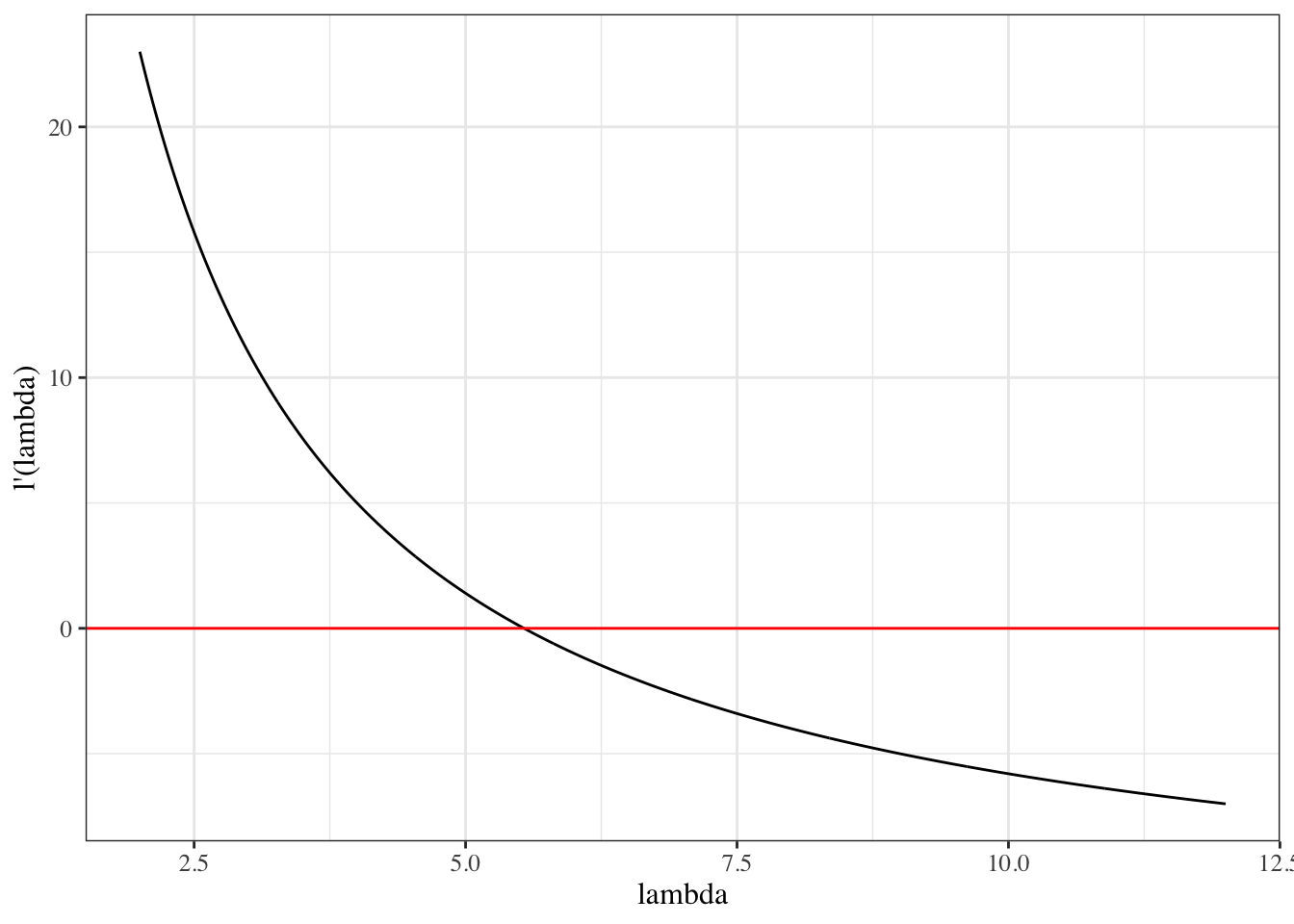
Exercise F.11 Graph the score function.

Solution.

Show R code

score = function(lambda, y = cyclones$number, n = length(y))
{
  (sum(y) / lambda) - n
}

ggplot() +
geom_function(fun = score, n = 1001) +
xlim(min(cyclones$number), max(cyclones$number)) +

ylab("l'(lambda)") +
xlab('lambda') +
geom_hline(yintercept = 0, col = 'red')
Figure F.5: score function of Dobson cyclone data

The Hessian matrix

Exercise F.12 Derive the Hessian matrix.

Solution. The Hessian function for an iid sample is the 2nd derivative(s) of the log-likelihood:

\[ \begin{aligned} \ell''( \lambda; \tilde{x} ) &= \frac{\partial}{\partial \lambda}\left(\frac{1}{\lambda} \sum_{i = 1}^nx_i- n\right)\\ &= \frac{\partial}{\partial \lambda}\frac{1}{\lambda} \sum_{i = 1}^nx_i- \frac{\partial}{\partial \lambda}n\\ &= -\frac{1}{\lambda^2} \sum_{i = 1}^nx_i\\ &= -\frac{1}{\lambda^2} n \bar x \\&= -\frac{1}{\lambda^2} \cdot 72 \end{aligned} \]

Exercise F.13 Graph the Hessian.

Solution.

Show R code

hessian = function(lambda, y = cyclones$number, n = length(y))
{
-sum(y)/(lambda^2)
}

ggplot() +
geom_function(fun = hessian, n = 1001) +
xlim(min(cyclones$number), max(cyclones$number)) +

ylab("l''(lambda)") +
xlab('lambda') +
geom_hline(yintercept = 0, col = 'red')
Figure F.6: Hessian function of Dobson cyclone data

Exercise F.14 Write the score equation (estimating equation).

Solution. \[\ell'( \lambda; \tilde{x} ) = 0\]

Exercise F.15 Solve the estimating equation for \(\lambda\):

Solution. \[ \begin{aligned} 0 &= \frac{1}{\lambda}\sum_{i = 1}^nx_i - n\\ n &= \frac{1}{\lambda}\sum_{i = 1}^nx_i\\ n\lambda &= \sum_{i = 1}^nx_i\\ \lambda &= \frac{1}{n}\sum_{i = 1}^nx_i\\ &=\bar x \end{aligned} \]

Let’s call this solution of the estimating equation \(\tilde \lambda\) for now:

\[\tilde \lambda \stackrel{\text{def}}{=}\bar x\]

Exercise F.16 Confirm that the Hessian \(\ell''(\lambda; \tilde{x})\) is negative when evaluated at \(\tilde \lambda\).

Solution. \[ \begin{aligned} \ell''( \tilde\lambda; \tilde{x} ) &= -\frac{1}{\tilde\lambda^2} n \bar x\\ &= -\frac{1}{\bar x^2} n\bar x\\ &= -\frac{n}{\bar x}\\ &<0\\ \end{aligned} \]

Exercise F.17 Find the MLE of \(\lambda\).

Solution. Since \(\ell''(\tilde \lambda; \tilde{x})<0\), \(\tilde \lambda\) is at least a local maximizer of the likelihood function \(\mathcal L(\lambda)\). Since there is only one solution to the estimating equation and the Hessian is negative definite everywhere, \(\tilde \lambda\) must also be the global maximizer of \(\mathcal L(\lambda; \tilde{x})\):

Show R code
mle = mean(cyclones$number)

\[\hat{\lambda}_{\text{ML}} = \bar x = 5.5385\]

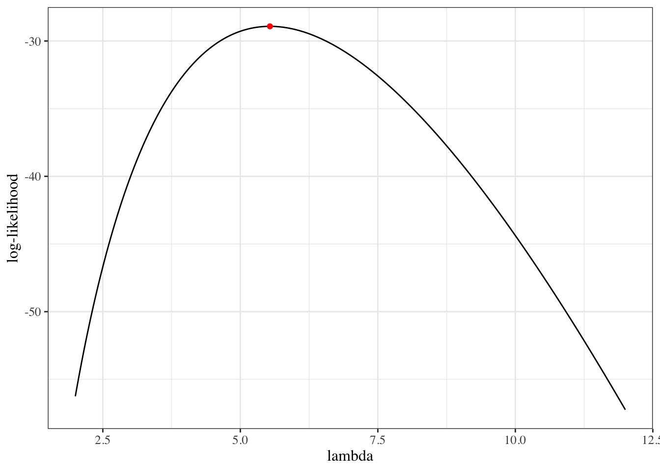
Exercise F.18 Graph the log-likelihood with the MLE superimposed.

Solution.

Show R code
library(dplyr)

mle_data = tibble(x = mle, y = loglik(mle))
ll_plot + geom_point(data = mle_data, aes(x = x, y = y), col = 'red')
Figure F.7: log-likelihood of Dobson cyclone data with MLE

Information matrices

Show R code
obs_inf = function(...) -hessian(...)
ggplot() +
geom_function(fun = obs_inf, n = 1001) +
xlim(min(cyclones$number), max(cyclones$number)) +
ylab("I(lambda)") +
xlab('lambda') +
geom_hline(yintercept = 0, col = 'red') 
Figure F.8: Observed information function of Dobson cyclone data

Example F.1 (Finding the MLE using the Newton-Raphson algorithm)  

We found that the MLE was \(\hat{\lambda} = \bar{x}\), by solving the score equation \(\ell'(\lambda)=0\) for \(\lambda\).

What if we hadn’t been able to solve the score equation?

Then we could start with some initial guess \({\widehat{\lambda}}^*\), such as \({\widehat{\lambda}}^*= 3\), and use the Newton-Raphson algorithm.

Show R code
# specify initial guess:
cur_lambda_est = 3

In Exercise F.10, we found that the score function was:

\[ \ell'( \lambda; \tilde{x} ) = \left(\frac{72}{\lambda} \right) - n \]

In Exercise F.12, we found that the Hessian was:

\[ \ell''( \lambda; \tilde{x} ) = -\frac{72}{\lambda^2} \]


So we can approximate the the score function using the first-order Taylor polynomial:

\[ \begin{aligned} \ell'(\lambda) &\approx \ell'^*(\lambda) \\ &\stackrel{\text{def}}{=}\ell'({\widehat{\lambda}}^*) + \ell''({\widehat{\lambda}}^*)(\lambda - {\widehat{\lambda}}^*) \\ &= \left(\frac{72}{{\widehat{\lambda}}^*} - n\right) + \left(-\frac{72}{\left({\widehat{\lambda}}^*\right)^2}\right) (\lambda - {\widehat{\lambda}}^*) \end{aligned} \]


Figure F.9 compares the true score function and the approximate score function at \({\widehat{\lambda}}^*= 3\).

Show R code
approx_score = function(lambda, lhat, ...)
{
  score(lambda = lhat, ...) +
  hessian(lambda = lhat, ...) * (lambda - lhat)
}

point_size = 5

plot1 = ggplot() +
geom_function(
  fun = score, 
  aes(col = "true score function"), 
  n = 1001) +
geom_function(
  fun = approx_score, 
  aes(col = "approximate score function"),
  n = 1001, 
  args = list(lhat = cur_lambda_est)) +
geom_point(
  size = point_size,
  aes(x = cur_lambda_est, y = score(lambda = cur_lambda_est),
      col = "current estimate")
) +
geom_point(
size = point_size,
aes(
x = xbar,
y = 0,
col = "true MLE"
)
) +
xlim(min(cyclones$number), max(cyclones$number)) +
ylab("l'(lambda)") +
xlab('lambda') +
geom_hline(yintercept = 0)

print(plot1)
Figure F.9: score function of Dobson cyclone data and approximate score function

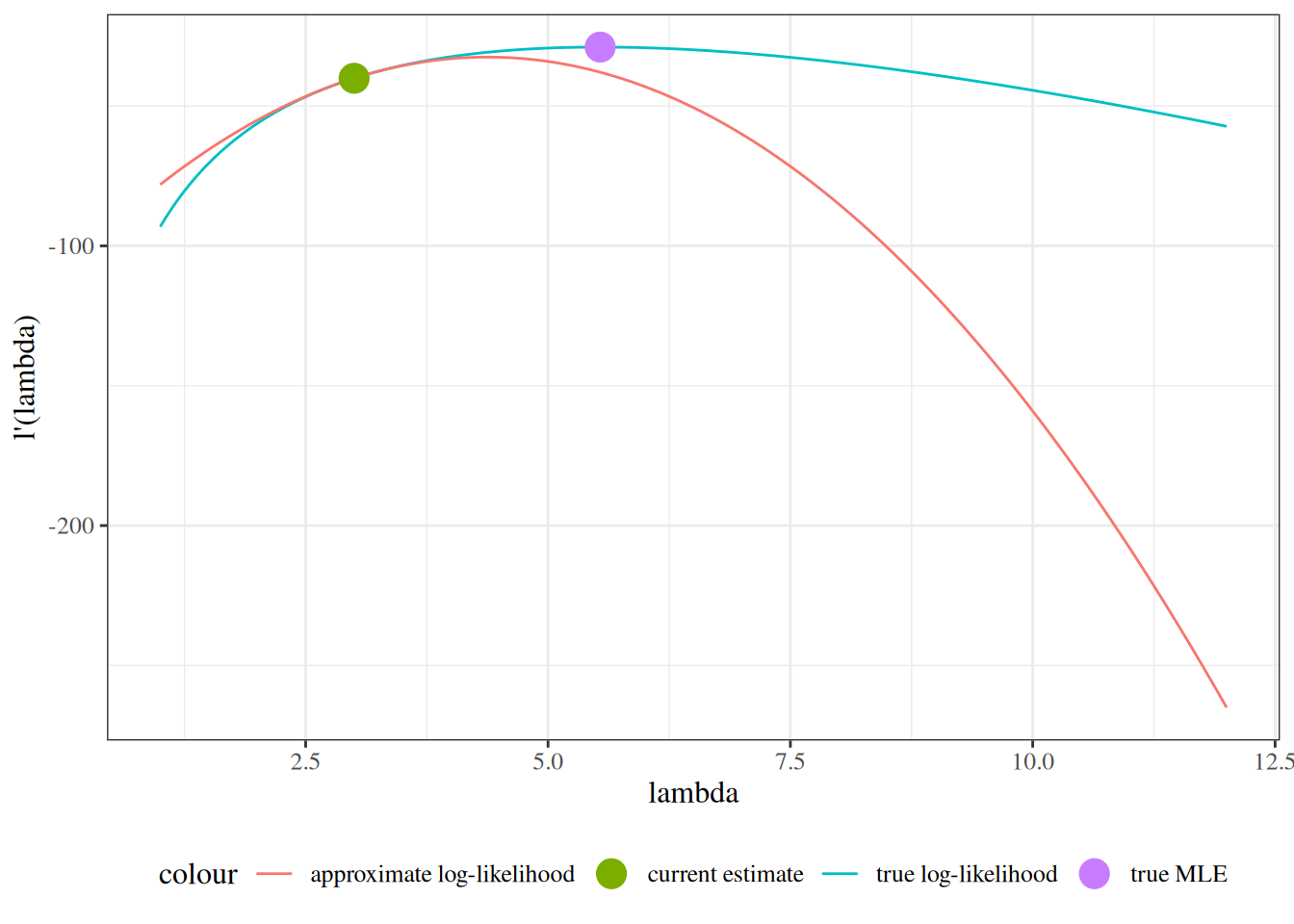
This is equivalent to estimating the log-likelihood with a second-order Taylor polynomial:

\[ \ell^*(\lambda) = \ell({\widehat{\lambda}}^*) + (\lambda - {\widehat{\lambda}}^*) \ell'({\widehat{\lambda}}^*) + \frac{1}{2}\ell''({\widehat{\lambda}}^*)(\lambda-{\widehat{\lambda}}^*)^2 \]

Show R code
approx_loglik = function(lambda, lhat, ...)
{
loglik(lambda = lhat, ...) +
score(lambda = lhat, ...) * (lambda - lhat) +
  1/2 * hessian(lambda = lhat, ...) * (lambda - lhat)^2
}

plot_loglik = ggplot() +
geom_function(
  fun = loglik, 
  aes(col = "true log-likelihood"), 
  n = 1001) +
geom_function(
  fun = approx_loglik, 
  aes(col = "approximate log-likelihood"),
  n = 1001, 
  args = list(lhat = cur_lambda_est)) +
geom_point(
  size = point_size,
  aes(x = cur_lambda_est, y = loglik(lambda = cur_lambda_est),
      col = "current estimate")
) +
geom_point(
size = point_size,
aes(
x = xbar,
y = loglik(xbar),
col = "true MLE"
)
) +
xlim(min(cyclones$number) - 1, max(cyclones$number)) +
ylab("l'(lambda)") +
xlab('lambda')

print(plot_loglik)
Figure F.10: log-likelihood of Dobson cyclone data and approximate log-likelihood function

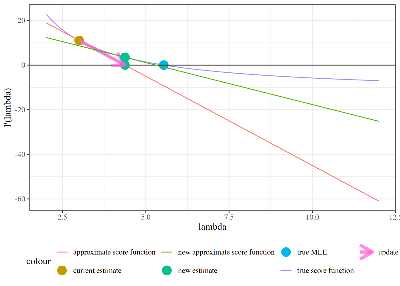
The approximate score function, \(\ell'^*(\lambda)\), is a linear function of \(\lambda\), so it is easy to solve the corresponding approximate score equation, \(\ell'^*(\lambda) = 0\), for \(\lambda\):

\[ \begin{aligned} \lambda &= {\widehat{\lambda}}^*- \ell'({\widehat{\lambda}}^*) \cdot\left(\ell''({\widehat{\lambda}}^*)\right)^{-1} \\ &= 4.375 \end{aligned} \]

Show R code
new_lambda_est <- 
   cur_lambda_est - 
   score(cur_lambda_est) * hessian(cur_lambda_est)^-1

Show R code
plot2 = plot1 +
  geom_point(size = point_size,
             aes(x = new_lambda_est,
                 y = 0,
                 col = "new estimate")) +
  geom_segment(
    arrow = grid::arrow(),
    linewidth = 2,
    alpha = .7,
    aes(
      x = cur_lambda_est,
      y = approx_score(lhat = cur_lambda_est,
                       lambda = cur_lambda_est),
      xend = new_lambda_est,
      yend = 0,
      col = "update"
    )
  )
print(plot2)
Figure F.11: score function of Dobson cyclone data and approximate score function

So we update \({\widehat{\lambda}}^*\leftarrow 4.375\) and repeat our estimation process:

Show R code
plot2 +
geom_function(
  fun = approx_score, 
  aes(col = "new approximate score function"),
  n = 1001, 
  args = list(lhat = new_lambda_est)) +
geom_point(
  size = point_size,
  aes(x = new_lambda_est, y = score(lambda = new_lambda_est),
      col = "new estimate")
)
Figure F.12: score function of Dobson cyclone data and approximate score function

We repeat this process until the likelihood converges:

Show R code

library(tibble)
cur_lambda_est = 3 # restarting
diff_loglik = Inf
tolerance = 10 ^ -4
max_iter = 100
NR_info = tibble(
  iteration = 0,
  lambda = cur_lambda_est |> num(digits = 4),
  likelihood = lik(cur_lambda_est),
  `log(likelihood)` = loglik(cur_lambda_est)  |> num(digits = 4),
  score = score(cur_lambda_est),
  hessian = hessian(cur_lambda_est)
)

for (cur_iter in 1:max_iter)
{
  new_lambda_est <-
    cur_lambda_est - score(cur_lambda_est) * hessian(cur_lambda_est) ^ -1
  
  diff_loglik = loglik(new_lambda_est) - loglik(cur_lambda_est)
  
  new_NR_info = tibble(
    iteration = cur_iter,
    lambda = new_lambda_est,
    likelihood = lik(new_lambda_est),
    `log(likelihood)` = loglik(new_lambda_est),
    score = score(new_lambda_est),
    hessian = hessian(new_lambda_est),
    `diff(loglik)` = diff_loglik
  )
  
  NR_info = NR_info |> bind_rows(new_NR_info)
  
  cur_lambda_est = new_lambda_est
  
  if (abs(diff_loglik) < tolerance)
    break
  
}

NR_info
Table F.3: Convergence of Newton-Raphson Algorithm for finding MLE of cyclone data

Compare with Exercise F.17


Show R code
ll_plot +
  geom_segment(
    data = NR_info,
    arrow = grid::arrow(),
    # linewidth = 2,
    alpha = .7,
    aes(
      x = lambda,
      xend = lead(lambda),
      y = `log(likelihood)`,
      yend = lead(`log(likelihood)`),
      col = factor(iteration)
    )
  )
Figure F.13: Newton-Raphson algorithm for finding MLE of model F.6 for cyclone data

F.3 Maximum likelihood inference for univariate Gaussian models

Suppose \(X_{1}, ..., X_{n} \ \sim_{\text{iid}}\ N(\mu, \sigma^{2})\). Let \(X = (X_{1},\ldots,X_{n})^{\top}\) be these random variables in vector format. Let \(x_{i}\) and \(x\) denote the corresponding observed data. Then \(\theta = (\mu,\sigma^{2})\) is the vector of true parameters, and \(\Theta = (\text{M}, \Sigma^2)\) is the vector of parameters as a random vector.

Then the log-likelihood is:

\[ \begin{aligned} \ell &\propto - \frac{n}{2}\text{log}\left\{\sigma^{2}\right\} - \frac{1}{2}\sum_{i = 1}^{n}\frac{( x_{i} - \mu)^{2}}{\sigma^{2}}\\ &= - \frac{n}{2}\text{log}\left\{\sigma^{2}\right\} - \frac{1}{2\sigma^{2}}\sum_{i = 1}^{n}{x_{i}^{2} - 2x_{i}\mu + \mu^{2}} \end{aligned} \]

F.3.1 The score function

\[\ell'(x,\theta) \stackrel{\text{def}}{=}\frac{\partial}{\partial \theta}\ell(x,\theta) = \left( \begin{array}{r} \frac{\partial}{\partial \mu}\ell(\theta;x) \\ \frac{\partial}{\partial \sigma^{2}}\ell(\theta;x) \end{array} \right) = \left( \begin{array}{r} \ell_{\mu}'(\theta;x) \\ \ell_{\sigma^{2}}'(\theta;x) \end{array} \right)\].

\(\ell'(x,\theta)\) is the function we set equal to 0 and solve to find the MLE:

\[{\widehat{\theta}}_{ML} = \left\{ \theta:\ell'(x,\theta) = 0 \right\}\]

F.3.2 MLE of \(\mu\)

\[ \begin{aligned} \frac{d\ell}{d\mu} &= - \frac{1}{2}\sum_{i = 1}^{n} \frac{- 2(x_{i} - \mu)}{\sigma^{2}} \\ &= \frac{1}{\sigma^{2}} \left[ \left( \sum_{i = 1}^{n}x_{i} \right) - n\mu \right] \end{aligned} \]

If \(\frac{d\ell}{d\mu} = 0\), then \(\mu = \overline{x} \stackrel{\text{def}}{=}\frac{1}{n}\sum_{i = 1}^{n}x_{i}\).

\[\frac{d^{2}\ell}{(d\mu)^{2}} = \frac{- n}{\sigma^{2}} < 0\]

So \({\widehat{\mu}}_{ML} = \overline{x}\).

F.3.3 MLE of \(\sigma^{2}\)

Reparametrizing the Gaussian distribution

When solving for \({\widehat{\sigma}}_{ML}\), you can treat \(\sigma^{2}\) as an atomic variable (don’t differentiate with respect to \(\sigma\) or things get messy). In fact, you can replace \(\sigma^{2}\) with \(1/\tau\) and differentiate with respect to \(\tau\) instead, and the process might be even easier.

\[\frac{d\ell}{d\sigma^{2}} = \frac{\partial}{\partial \sigma^{2}}\left( - \frac{n}{2}\text{log}\left\{\sigma^{2}\right\} - \frac{1}{2}\sum_{i = 1}^{n}\frac{\left( x_{i} - \mu \right)^{2}}{\sigma^{2}} \right)\ \]

\[= - \frac{n}{2}\left( \sigma^{2} \right)^{- 1} + \frac{1}{2}\left( \sigma^{2} \right)^{- 2}\sum_{i = 1}^{n}\left( x_{i} - \mu \right)^{2}\]

If \(\frac{d\ell}{d\sigma^{2}} = 0\), then:

\[\frac{n}{2}\left( \sigma^{2} \right)^{- 1} = \frac{1}{2}\left( \sigma^{2} \right)^{- 2}\sum_{i = 1}^{n}\left( x_{i} - \mu \right)^{2}\]

\[\sigma^{2} = \frac{1}{n}\sum_{i = 1}^{n}\left( x_{i} - \mu \right)^{2}\]

We plug in \({\widehat{\mu}}_{ML} = \overline{x}\) to maximize globally (a technique called profiling):

\[\sigma_{ML}^{2} = \frac{1}{n}\sum_{i = 1}^{n}\left( x_{i} - \overline{x} \right)^{2}\]

Now:

\[ \begin{aligned} \frac{d^{2}\ell}{\left( d\sigma^{2} \right)^{2}} &= \frac{\partial}{\partial \sigma^{2}}\left\{ - \frac{n}{2}\left( \sigma^{2} \right)^{- 1} + \frac{1}{2}\left( \sigma^{2} \right)^{- 2}\sum_{i = 1}^{n}\left( x_{i} - \mu \right)^{2} \right\}\\ &= \left\{ - \frac{n}{2}\frac{\partial}{\partial \sigma^{2}}\left( \sigma^{2} \right)^{- 1} + \frac{1}{2}\frac{\partial}{\partial \sigma^{2}}\left( \sigma^{2} \right)^{- 2}\sum_{i = 1}^{n}\left( x_{i} - \mu \right)^{2} \right\}\\ &= \left\{ \frac{n}{2}\left( \sigma^{2} \right)^{- 2} - \left( \sigma^{2} \right)^{- 3}\sum_{i = 1}^{n}\left( x_{i} - \mu \right)^{2} \right\}\\ &= \left( \sigma^{2} \right)^{- 2}\left\{ \frac{n}{2} - \left( \sigma^{2} \right)^{- 1}\sum_{i = 1}^{n}\left( x_{i} - \mu \right)^{2} \right\} \end{aligned} \]

Evaluated at \(\mu = \overline{x},\sigma^{2} = \frac{1}{n}\sum_{i = 1}^{n}\left( x_{i} - \overline{x} \right)^{2}\), we have:

\[ \begin{aligned} \frac{d^{2}\ell}{\left( d\sigma^{2} \right)^{2}} &= \left( {\widehat{\sigma}}^{2} \right)^{- 2}\left\{ \frac{n}{2} - \left( {\widehat{\sigma}}^{2} \right)^{- 1}\sum_{i = 1}^{n}\left( x_{i} - \overline{x} \right)^{2} \right\}\\ &= \left( {\widehat{\sigma}}^{2} \right)^{- 2}\left\{ \frac{n}{2} - \left( {\widehat{\sigma}}^{2} \right)^{- 1}n{\widehat{\sigma}}^{2} \right\}\\ &= \left( {\widehat{\sigma}}^{2} \right)^{- 2}\left\{ \frac{n}{2} - n \right\}\\ &= \left( {\widehat{\sigma}}^{2} \right)^{- 2}n\left\{ \frac{1}{2} - 1 \right\}\\ &= \left( {\widehat{\sigma}}^{2} \right)^{- 2}n\left( - \frac{1}{2} \right) < 0 \end{aligned} \]

Finally, we have:

\[ \begin{aligned} \frac{d^{2}\ell}{d\mu\ d\sigma^{2}} &= \frac{\partial}{\partial \mu}\left\{ - \frac{n}{2}\left( \sigma^{2} \right)^{- 1} + \frac{1}{2}\left( \sigma^{2} \right)^{- 2}\sum_{i = 1}^{n}\left( x_{i} - \mu \right)^{2} \right\}\\ &= \frac{1}{2}\left( \sigma^{2} \right)^{- 2}\frac{\partial}{\partial \mu}\sum_{i = 1}^{n}\left( x_{i} - \mu \right)^{2}\\ &= \frac{1}{2}\left( \sigma^{2} \right)^{- 2}\sum_{i = 1}^{n}{- 2(x_{i} - \mu)}\\ &= - \left( \sigma^{2} \right)^{- 2}\sum_{i = 1}^{n}{(x_{i} - \mu)} \end{aligned} \]

Evaluated at \(\mu = \widehat{\mu} = \overline{x},\sigma^{2} = {\widehat{\sigma}}^{2} = \frac{1}{n}\sum_{i = 1}^{n}\left( x_{i} - \overline{x} \right)^{2}\), we have:

\[\frac{d^{2}\ell}{d\mu\ d\sigma^{2}} = - \left( {\widehat{\sigma}}^{2} \right)^{- 2}\left( n\overline{x} - n\overline{x} \right) = 0\]

F.3.4 Covariance matrix

\[I = \begin{bmatrix} \frac{n}{\sigma^{2}} & 0 \\ 0 & \left( {\widehat{\sigma}}^{2} \right)^{- 2}n\left( - \frac{1}{2} \right) \end{bmatrix} = \begin{bmatrix} a & 0 \\ 0 & d \end{bmatrix}\]

So:

\[I^{- 1} = \frac{1}{ad}\begin{bmatrix} d & 0 \\ 0 & a \end{bmatrix} = \begin{bmatrix} \frac{1}{a} & 0 \\ 0 & \frac{1}{d} \end{bmatrix}\]

\[I^{- 1} = \begin{bmatrix} \frac{{\widehat{\sigma}}^{2}}{n} & 0 \\ 0 & \frac{{2\left( {\widehat{\sigma}}^{2} \right)}^{2}}{n} \end{bmatrix}\]

See Casella and Berger (2002) p322, example 7.2.12.

To prove it’s a maximum, we need:

  • \(\ell' = 0\)

  • At least one diagonal element of \(\ell''\) is negative.

  • Determinant of \(\ell''\) is positive.

F.4 Example: hormone therapy study

Now, we’re going to analyze some real-world data using a Gaussian model, and then we’re going to do a simulation to examine the properties of maximum likelihood estimation for that Gaussian model.

Here we look at the “heart and estrogen/progestin study” (HERS), a clinical trial of hormone therapy for prevention of recurrent heart attacks and death among 2,763 post-menopausal women with existing coronary heart disease (CHD) (Hulley et al. 1998).

We are going to model the distribution of fasting glucose among nondiabetics who don’t exercise.

Show R code
# load the data directly from a UCSF website
hers = haven::read_dta(
  paste0( # I'm breaking up the url into two chunks for readability
    "https://regression.ucsf.edu/sites/g/files",
    "/tkssra6706/f/wysiwyg/home/data/hersdata.dta"
  )
)
Show R code
hers |> head()
Table F.4: HERS dataset

Show R code

n.obs = 100 # we're going to take a small subset of the data to look at; 
# if we took the whole data set, the likelihood function would be hard to 
# graph nicely

library(dplyr)
data1 = 
  hers |> 
  filter(
    diabetes == 0,
    exercise == 0) |> 
  head(n.obs)

glucose_data = 
  data1 |> 
  pull(glucose)

library(ggplot2)
library(ggeasy)
plot1 = 
  data1 |> 
  ggplot(aes(x = glucose)) +
  geom_histogram(aes(x = glucose, after_stat(density))) +
  theme_classic() +
  easy_labs()

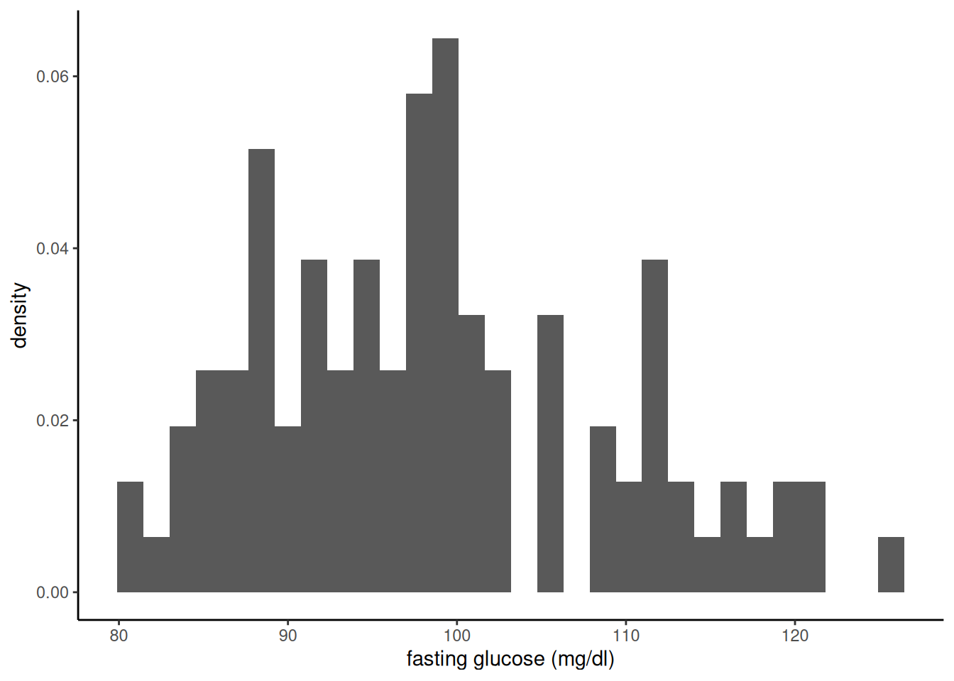
print(plot1)

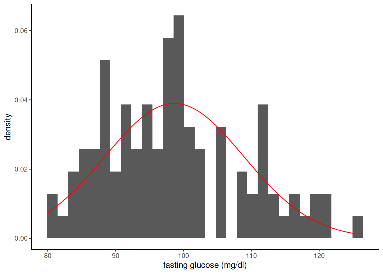
Looks somewhat plausibly Gaussian. Good enough for this example!

F.4.1 Find the MLEs

Show R code

mu_hat = mean(glucose_data)
sigma_sq_hat = mean((glucose_data - mean(glucose_data))^2)

Our MLEs are:

  • \(\hat\mu = 98.66\)

  • \(\hat\sigma^2 = 104.7444\)

Here’s the estimated distribution, superimposed on our histogram:

Show R code

plot1 +
  geom_function(
    fun = function(x) dnorm(x, mean = mu_hat, sd = sqrt(sigma_sq_hat)),
    col = "red"
  )

Looks like a somewhat decent fit? We could probably do better, but that’s for another time.

F.4.2 Construct the likelihood and log-likelihood functions

it’s often computationally more effective to construct the log-likelihood first and then exponentiate it to get the likelihood

Show R code

loglik = function(
    mu, # I'm assigning default values, which the function will use 
    # unless we tell it otherwise
    sigma = sd(x), # note that you can define some defaults based on other arguments
    x = glucose_data, 
    n = length(x)
)
{
  
  normalizing_constants = -n/2 * log((sigma^2) * 2 * pi) 
  
  likelihood_kernel = - 1/(2 * sigma^2) * 
    {
      # I have to do this part in a somewhat complicated way
      # so that we can pass in vectors of possible values of mu
      # and get the likelihood for each value;
      # for the binomial case it's easier
      sum(x^2) - 2 * sum(x) * mu + n * mu^2
    }
  
  answer = normalizing_constants + likelihood_kernel
  
  return(answer)
  
}

# `...` means pass any inputs to lik() along to loglik()
lik = function(...) exp(loglik(...))

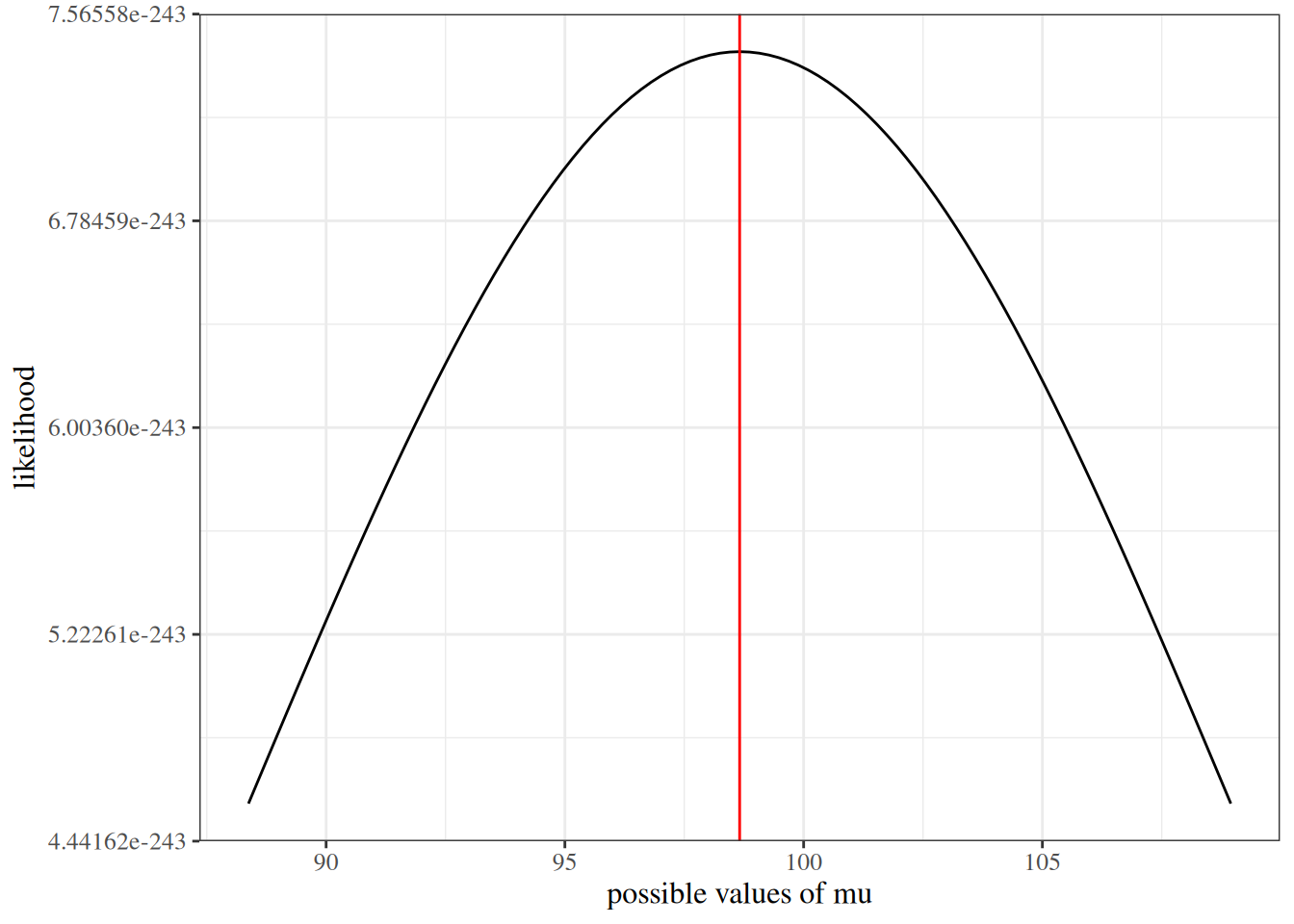
F.4.3 Graph the Likelihood as a function of \(\mu\)

(fixing \(\sigma^2\) at \(\hat\sigma^2 = 104.7444\))

Show R code

ggplot() + 
  geom_function(fun = function(x) lik(mu = x, sigma = sigma_sq_hat)) + 
  xlim(mean(glucose_data) + c(-1,1) * sd(glucose_data)) +
  xlab("possible values of mu") +
  ylab("likelihood") + 
  geom_vline(xintercept = mean(glucose_data), col = "red")

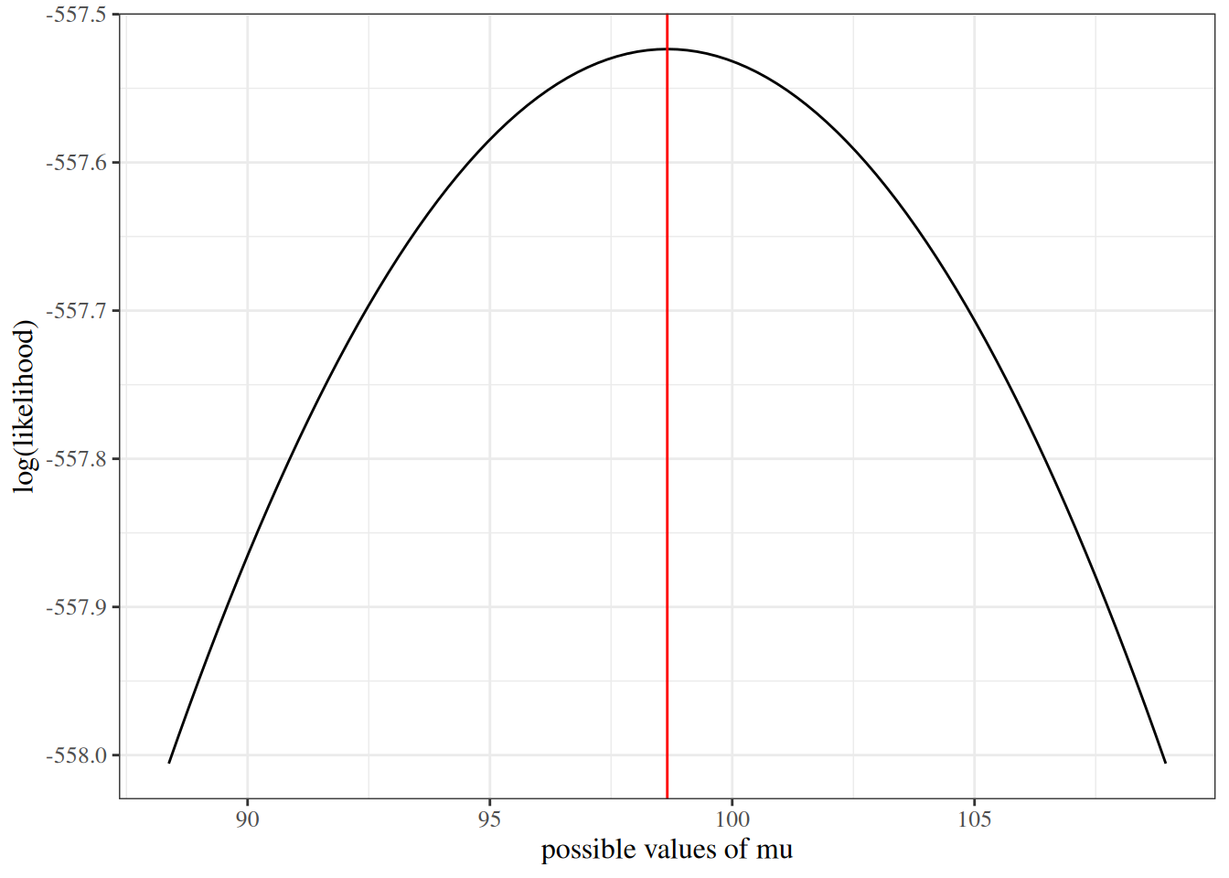
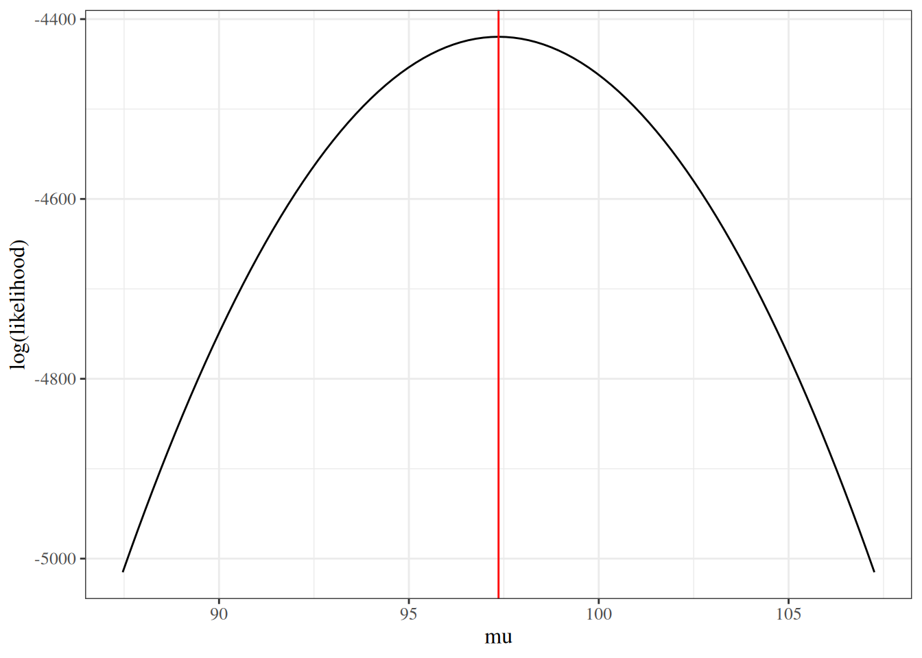
F.4.4 Graph the Log-likelihood as a function of \(\mu\)

(fixing \(\sigma^2\) at \(\hat\sigma^2 = 104.7444\))

Show R code

ggplot() + 
  geom_function(fun = function(x) loglik(mu = x, sigma = sigma_sq_hat)) + 
  xlim(mean(glucose_data) + c(-1,1) * sd(glucose_data)) +
  xlab("possible values of mu") +
  ylab('log(likelihood)') + 
  geom_vline(xintercept = mean(glucose_data), col = "red")

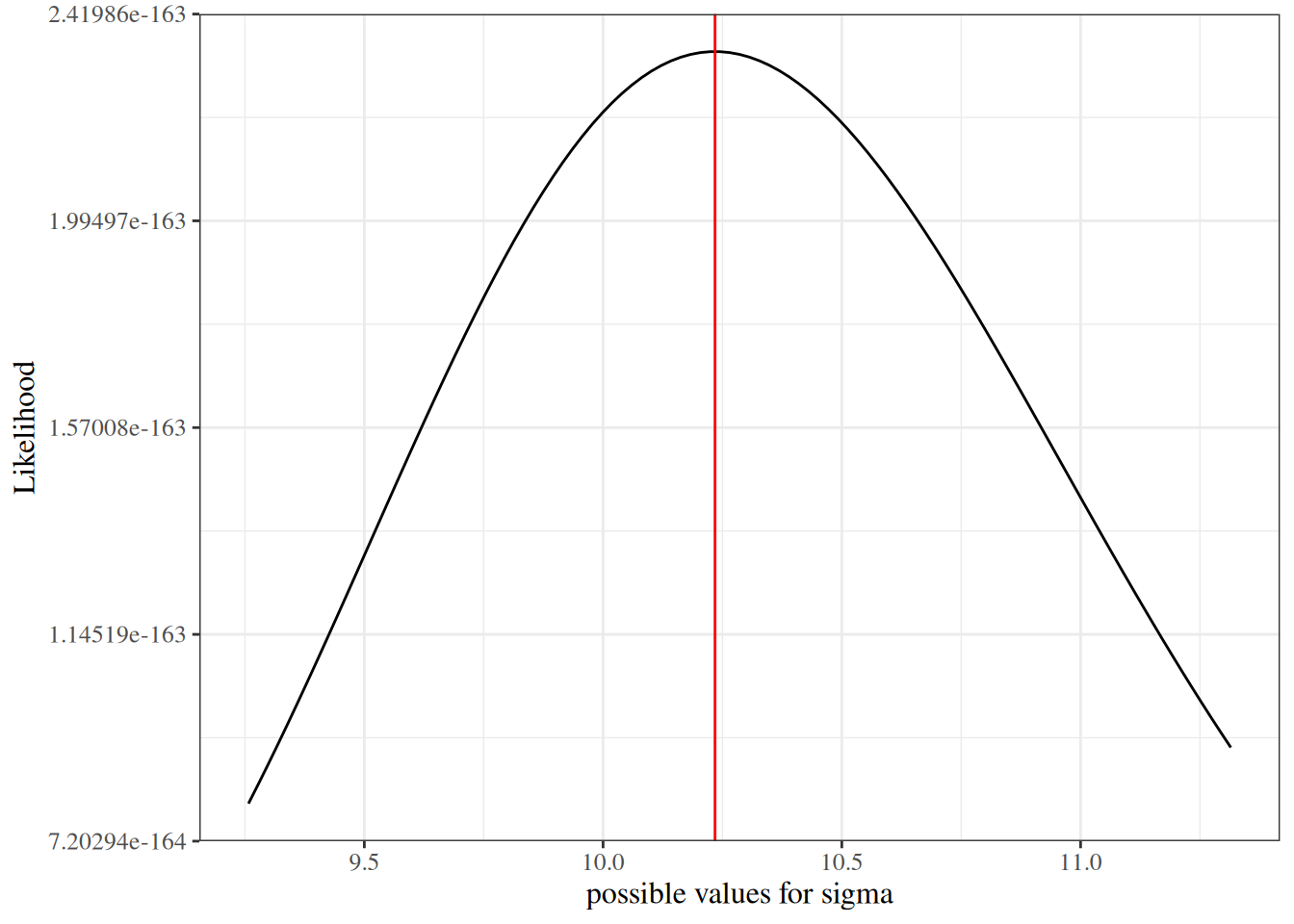
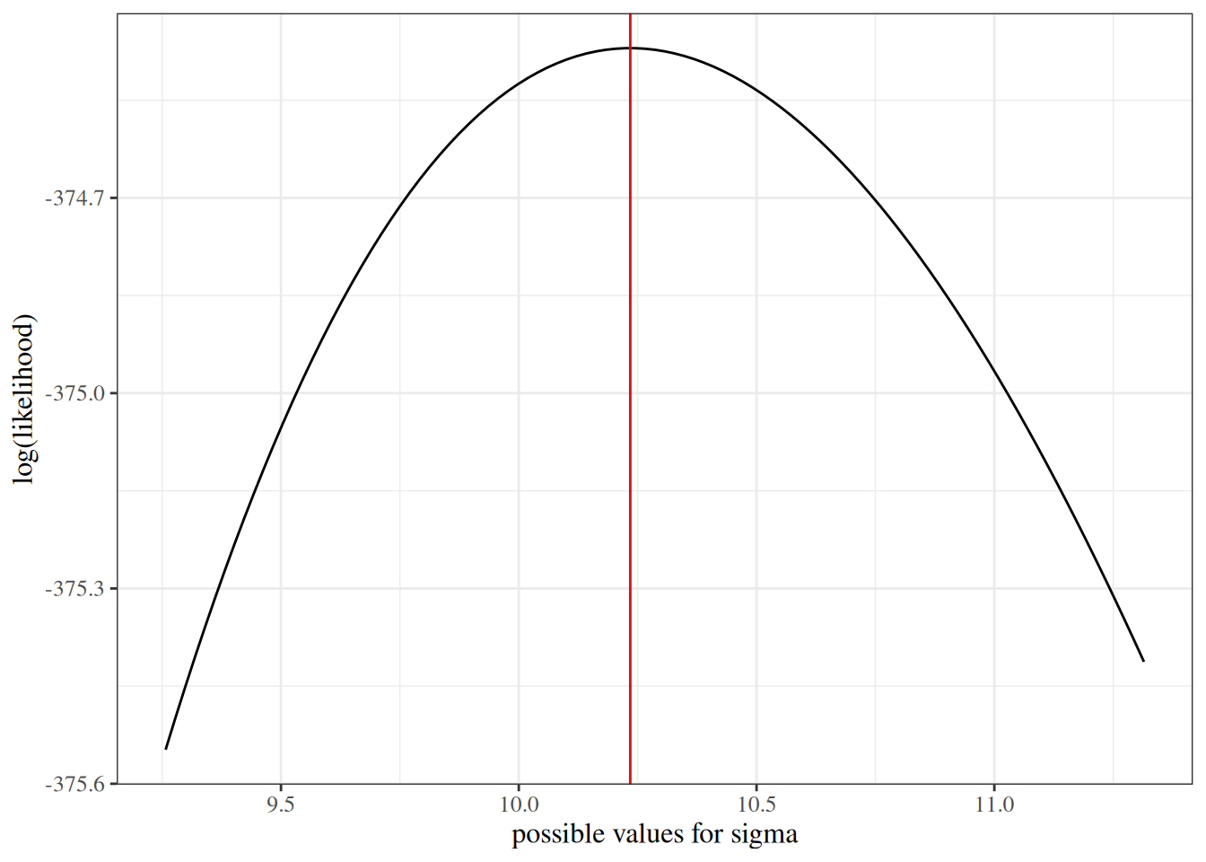
F.4.5 Likelihood and log-likelihood for \(\sigma\), conditional on \(\mu = \hat\mu\):

Show R code


ggplot() + 
  geom_function(fun = function(x) lik(sigma = x, mu = mean(glucose_data))) + 
  xlim(sd(glucose_data) * c(.9,1.1)) + 
  geom_vline(
    xintercept = sd(glucose_data) * sqrt(n.obs - 1)/sqrt(n.obs), 
    col = "red") +
  xlab("possible values for sigma") +
  ylab('Likelihood')

Show R code

ggplot() + 
  geom_function(
    fun = function(x) loglik(sigma = x, mu = mean(glucose_data))
  ) + 
  xlim(sd(glucose_data) * c(0.9, 1.1)) +
  geom_vline(
    xintercept = 
      sd(glucose_data) * sqrt(n.obs - 1) / sqrt(n.obs), 
    col = "red") +
  xlab("possible values for sigma") +
  ylab("log(likelihood)")

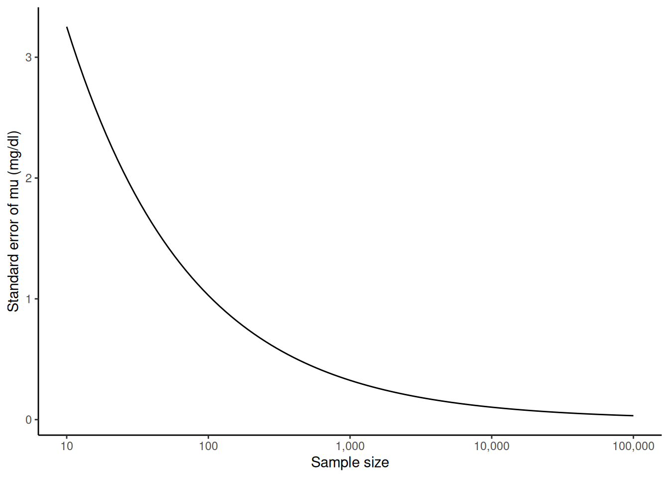
F.4.6 Standard errors by sample size:

Show R code

se.mu.hat = function(n, sigma = sd(glucose_data)) sigma/sqrt(n)
ggplot() + 
  geom_function(fun = se.mu.hat) + 
  scale_x_continuous(trans = "log10", limits = c(10, 10^5), name = "Sample size") +
  ylab("Standard error of mu (mg/dl)") +
  theme_classic()

F.4.7 Simulations

Create simulation framework

Here’s a function that performs a single simulation of a Gaussian modeling analysis:

Show R code

do_one_sim = function(
    n = 100,
    mu = mean(glucose_data),
    mu0 = mean(glucose_data) * 0.9,
    sigma2 = var(glucose_data), 
    return_data = FALSE # if this is set to true, we will create a list() containing both 
    # the analytic results and the vector of simulated data
)
{
  
  # generate data
  x = rnorm(n = 100, mean = mu, sd = sqrt(sigma2))
  
  # analyze data
  mu_hat = mean(x)
  sigmahat = sd(x)
  se_hat = sigmahat/sqrt(n)
  confint = mu_hat + c(-1, 1) * se_hat * qt(.975, df = n - 1)
  tstat = abs(mu_hat - mu0) / se_hat
  pval = pt(df = n - 1, q = tstat, lower = FALSE) * 2
  confint_covers = between(mu, confint[1], confint[2])
  test_rejects = pval < 0.05
  
  # if you want spaces, hyphens, or characters in your column names, use "", '', or ``:
  to_return = tibble(
    "mu-hat" = mu_hat,
    "sigma-hat" = sigmahat,
    "se_hat" = se_hat,
    "confint_left" = confint[1],
    "confint_right" = confint[2],
    "tstat" = tstat,
    "pval" = pval, 
    "confint covers true mu" = confint_covers,
    "test rejects null hypothesis" = test_rejects
  )
  
  if(return_data)
  {
    return(
      list(
        data = x, 
        results = to_return))
  } else
  {
    return(to_return)
  }
  
}

Let’s see what this function outputs for us:

Show R code

do_one_sim()

Looks good!

Now let’s check it against the t.test() function from the stats package:

Show R code

set.seed(1)
mu = mean(glucose_data)
mu0 = 80
sim.output = do_one_sim(mu0 = mu0, return_data = TRUE)
our_results = 
  sim.output$results |> 
  mutate(source = "`do_one_sim()`")

results_t.test = t.test(sim.output$data, mu = mu0)

results2 = 
  tibble(
    source = "`stats::t.test()`",
    "mu-hat" = results_t.test$estimate,
    "sigma-hat" = results_t.test$stderr*sqrt(length(sim.output$data)),
    "se_hat" = results_t.test$stderr,
    confint_left = results_t.test$conf.int[1],
    confint_right = results_t.test$conf.int[2],
    tstat = results_t.test$statistic,
    pval = results_t.test$p.value,
    "confint covers true mu" = between(mu, confint_left, confint_right),
     `test rejects null hypothesis` = pval < 0.05
  )

comparison = 
  bind_rows(
    our_results,
    results2
  ) |> 
  relocate(
    "source",
    .before = everything()
  )

comparison

Looks like we got it right!

Run 1000 simulations

Here’s a function that calls the previous function n_sims times and summarizes the results:

Show R code

do_n_sims = function(
    n_sims = 1000,
    ... # this symbol means "allow additional arguments to be passed on to the `do_sim_once` function
)
{
  
  sim_results = NULL # we're going to create a "tibble" of results, 
  # row by row (slightly different from the hint on the homework)
  
  for (i in 1:n_sims)
  {
    
    set.seed(i)
    
    current_results = 
      do_one_sim(...) |> # here's where the simulation actually gets run
      mutate(
        sim_number = i
      ) |> 
      relocate(sim_number, .before = everything())
    
    sim_results = 
      sim_results |> 
      bind_rows(current_results)
    
  }
  
  return(sim_results)
}
Show R code

sim_results = do_n_sims(
  n_sims = 100,
  mu = mean(glucose_data),
  sigma2 = var(glucose_data),  
  n = 100 # this is the number of samples per simulated data set
)

sim_results |> head(10)

The simulation results are in! Now we have to analyze them.

Analyze simulation results

To do that, we write another function:

Show R code

summarize_sim = function(
    sim_results, 
    mu = mean(glucose_data),
    sigma2 = var(glucose_data), 
    n = 100)
{
  
  
  # calculate the true standard error based on the data-generating parameters:
  `se(mu-hat)` = sqrt(sigma2/n)
  
  sim_results |> 
    summarize(
      `bias[mu-hat]` = mean(`mu-hat`) - mu,
      `SE(mu-hat)` = sd(`mu-hat`),
      `bias[SE-hat]` = mean(se_hat) - `se(mu-hat)`,
      `SE(SE-hat)` = sd(se_hat),
      coverage = mean(`confint covers true mu`),
      power = mean(`test rejects null hypothesis`)
    )
  
}

Let’s try it out:

Show R code

sim_summary = summarize_sim(
  sim_results, 
  mu = mean(glucose_data), 
  # this function needs to know the true parameter values in order to assess bias
  sigma2 = var(glucose_data), 
  n = 100)

sim_summary

From this simulation, we observe that our estimate of \(\mu\), \(\hat\mu\), has minimal bias, and so does our estimate of \(SE(\hat\mu)\), \(\hat{SE}(\hat\mu)\).

The confidence intervals captured the true value even more often than they were supposed to, and the hypothesis test always rejected the null hypothesis.

I wonder what would happen with a different sample size, a different true \(\mu\) value, or a different \(\sigma^2\) value…


  1. https://en.wikipedia.org/wiki/Does_exactly_what_it_says_on_the_tin↩︎

  2. a.k.a. the gradient↩︎

  3. I might sometimes switch the order of \(x,\) \(\theta\); this is unintentional and not meaningful.↩︎

  4. named after mathematician Otto Hesse↩︎