Appendix G — Introduction to Bayesian inference

---

---

Configuring R

Functions from these packages will be used throughout this document:

library(conflicted) # check for conflicting function definitions
# library(printr) # inserts help-file output into markdown output
library(rmarkdown) # Convert R Markdown documents into a variety of formats.
library(pander) # format tables for markdown
library(ggplot2) # graphics
library(ggeasy) # help with graphics
library(ggfortify) # help with graphics
library(dplyr) # manipulate data
library(tibble) # `tibble`s extend `data.frame`s
library(magrittr) # `%>%` and other additional piping tools
library(haven) # import Stata files
library(knitr) # format R output for markdown
library(tidyr) # Tools to help to create tidy data
library(plotly) # interactive graphics
library(dobson) # datasets from Dobson and Barnett 2018
library(parameters) # format model output tables for markdown
library(haven) # import Stata files
library(latex2exp) # use LaTeX in R code (for figures and tables)
library(fs) # filesystem path manipulations
library(survival) # survival analysis
library(survminer) # survival analysis graphics
library(KMsurv) # datasets from Klein and Moeschberger
library(parameters) # format model output tables for
library(webshot2) # convert interactive content to static for pdf
library(forcats) # functions for categorical variables ("factors")
library(stringr) # functions for dealing with strings
library(lubridate) # functions for dealing with dates and times

Here are some R settings I use in this document:

rm(list = ls()) # delete any data that's already loaded into R

conflicts_prefer(dplyr::filter)
ggplot2::theme_set(
  ggplot2::theme_bw() + 
        # ggplot2::labs(col = "") +
    ggplot2::theme(
      legend.position = "bottom",
      text = ggplot2::element_text(size = 12, family = "serif")))

knitr::opts_chunk$set(message = FALSE)
options('digits' = 6)

panderOptions("big.mark", ",")
pander::panderOptions("table.emphasize.rownames", FALSE)
pander::panderOptions("table.split.table", Inf)
conflicts_prefer(dplyr::filter) # use the `filter()` function from dplyr() by default
legend_text_size = 9

---

Suppose $X_1,...,X_n{\sim }_{\text{iid}}N(M,1)$

Suppose $M\sim N(0,1)$.

Then: $$\begin{array}{rl}p(M=\mu |X=x)& \propto p(M=\mu ,X=x)\\ & =p(X=x|M=\mu )p(M=\mu )\\ & \propto \text{exp}\{-\frac{1}{2}n{\mu }^2-2\mu n\overline{x}\}\text{exp}\{-\frac{1}{2}{\mu }^2\}\\ & =\text{exp}\{-\frac{1}{2}(n+1){\mu }^2-2\mu n\overline{x}\}\\ & \propto \text{exp}\{-\frac{1}{2}(n+1)(\mu -\frac{n}{n+1}\overline{x}{)}^2\}\end{array}$$ So: $$p(M=\mu |X=x)\sim N(\frac{n}{n+1}\overline{x},(n+1{)}^{-1})$$

Let’s put this in perspective.

Here’s a frequentist CI:

set.seed(1)
mu <- 2
sigma <- 1
n <- 20
x <- rnorm(n = n, mean = mu, sd = sigma)
xbar <- mean(x)
se <- sigma / sqrt(n)
CI_freq <- xbar + se * qnorm(c(.025, .975))
print(CI_freq)
#> [1] 1.75226 2.62879

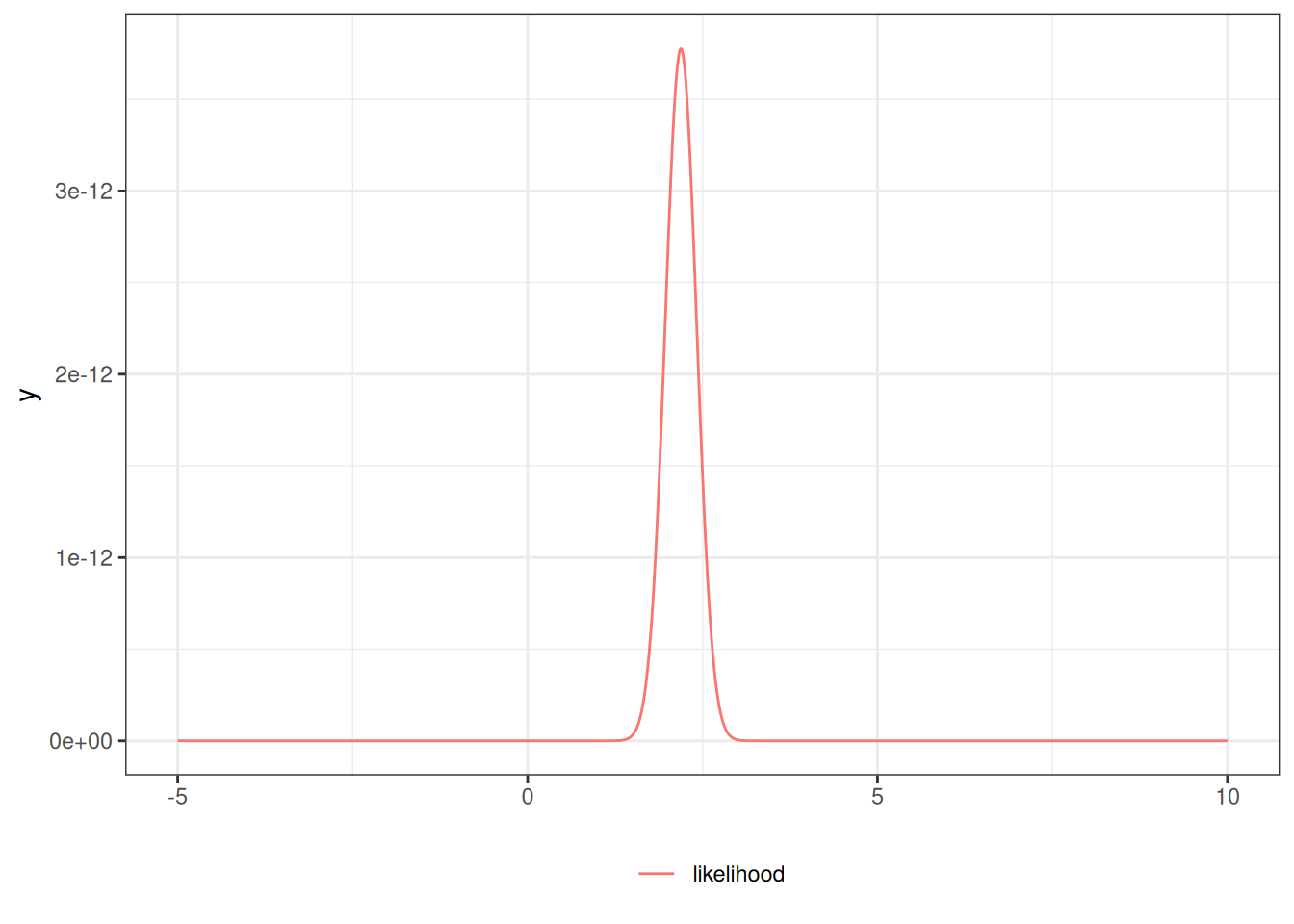
lik0 <- function(mu) dnorm(x = x, mean = mu, sd = 1) |> prod()
lik <- function(mu) {
  (2 * pi * sigma^2)^(-n / 2) *
    exp(
      -1 / (2 * sigma^2) *
        (sum(x^2) - 2 * mu * sum(x) + n * (mu^2))
    )
}
library(ggplot2)
ngraph <- 1001
plot1 <- ggplot() +
  geom_function(fun = lik, aes(col = "likelihood"), n = ngraph) +
  xlim(c(-5, 10)) +
  theme_bw() +
  labs(col = "") +
  theme(legend.position = "bottom")
print(plot1)

Here’s a Bayesian CI:

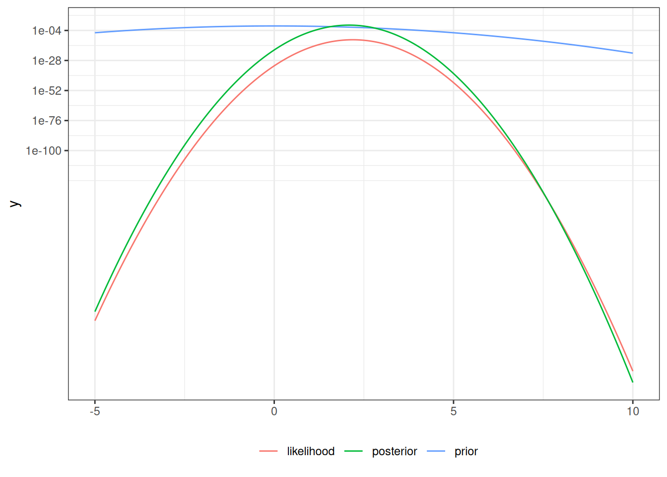
mu_prior_mean <- 0
mu_prior_sd <- 1
mu_post_mean <- n / (n + 1) * xbar
mu_post_var <- 1 / (n + 1)
mu_post_sd <- sqrt(mu_post_var)
CI_bayes <- qnorm(
  p = c(.025, .975),
  mean = mu_post_mean,
  sd = mu_post_sd
)
print(CI_bayes)
#> [1] 1.65851 2.51391
prior <- function(mu) dnorm(mu, mean = mu_prior_mean, sd = mu_prior_sd)
posterior <- function(mu) dnorm(mu, mean = mu_post_mean, sd = mu_post_sd)
plot2 <- plot1 +
  geom_function(fun = prior, aes(col = "prior"), n = ngraph) +
  geom_function(fun = posterior, aes(col = "posterior"), n = ngraph)
print(plot2 + scale_y_log10())

Here’s $p(M\in (l(x),r(x))|X=x)$:

pr_in_CI <- pnorm(
  CI_freq,
  mean = mu_post_mean,
  sd = mu_post_sd
) |> diff()
print(pr_in_CI)
#> [1] 0.930583

G.1 Other resources

UC Davis courses

• STA 145: “Bayesian Statistical Inference”
• ECL 234: “Bayesian Models - A Statistical Primer”
• PLS 207: “Applied Statistical Modeling for the Environmental Sciences”
• PSC 205H: “Applied Bayesian Statistics for Social Scientists”

Books

• (Ross 2022) is a free online textbook
• “Population health thinking with Bayesian networks” (Aragon 2018) is on my to-read list

Aragon, Tomas J. 2018. “Population Health Thinking with Bayesian Networks.” https://escholarship.org/uc/item/8000r5m5.

Ross, Kevin. 2022. An Introduction to Bayesian Reasoning and Methods. Online. https://bookdown.org/kevin_davisross/bayesian-reasoning-and-methods/.