rm(list =ls())# delete any data that's already loaded into Rconflicts_prefer(dplyr::filter)ggplot2::theme_set(ggplot2::theme_bw()+# ggplot2::labs(col = "") +ggplot2::theme( legend.position ="bottom", text =ggplot2::element_text(size =12, family ="serif")))knitr::opts_chunk$set(message =FALSE)options('digits'=6)panderOptions("big.mark", ",")pander::panderOptions("table.emphasize.rownames", FALSE)pander::panderOptions("table.split.table", Inf)conflicts_prefer(dplyr::filter)# use the `filter()` function from dplyr() by defaultlegend_text_size=9run_graphs=TRUE
1 Introduction
This chapter presents models for count data outcomes. With covariates, the event rate \(\lambda\) becomes a function of the covariates \(\tilde{X}= (X_1, \dots,X_n)\). Typically, count data models use a \(\text{log}{\left\{\right\}}\) link function, and thus an \(\text{exp}{\left\{\right\}}\) inverse-link function. That is:
In contrast with the other covariates (represented by \(\tilde{X}\)), \(t\) enters this expression with a \(\log{}\) transformation and without a corresponding \(\beta\) coefficient; in other words, \(\text{log}{\left\{t\right\}}\) is an offset term.
Exercise 2 What are the units of \(\mu\) in Equation 1?
SolutionSolution
Solution 2. \(\mu\) is the mean of \(Y\), and \(Y\) is a count, so \(\mu\) is also a count; for example:
3.1 cyclones,
10.23 ER visits
15.01 infections
Exercise 3 What are the units of \(\lambda\) in Equation 1?
SolutionSolution
Solution 3. \(\lambda = \mu/t\), so \(\lambda\) is a rate of counts per unit of \(t\). For example:
3.1 cyclones per year
2.023 ER visits per 10 person-years
15.01 infections per 1000 person-years at risk
2 Interpreting Poisson regression models
Differences on the log-rate scale become ratios on the rate scale, because
Therefore, according to this model, differences of \(\delta\) in covariate \(x_j\) correspond to rate ratios of \(\text{exp}{\left\{\beta_j \cdot \delta\right\}}\).
That is, letting \(\tilde{X}_{-j}\) denote vector \(\tilde{X}\) with element \(j\) removed:
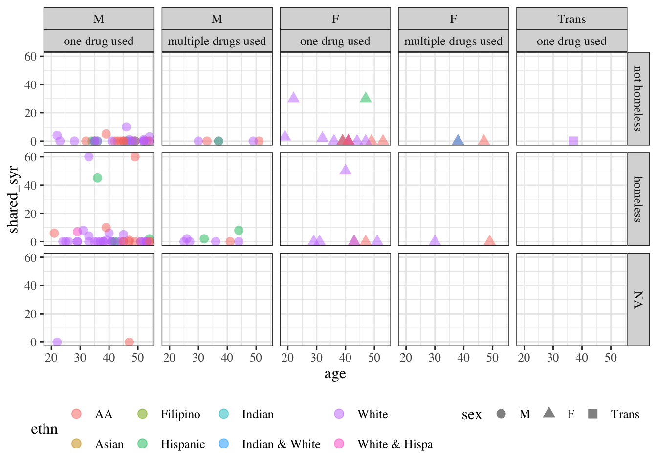
Table 3: Counts of observations in needles dataset by sex, unhoused status, and multiple drug use
Show R code
needles|>dplyr::select(sex, homeless, polydrug)|>summary()#> sex homeless polydrug #> M :97 not homeless:63 one drug used :109 #> F :30 homeless :61 multiple drugs used: 19 #> Trans: 1 NAs : 4
There’s only one individual with sex = Trans, which unfortunately isn’t enough data to analyze. We will remove that individual:
According to this model, if \(Z=1\), then \(Y\) will always be zero, regardless of \(X\) and \(T\):
\[P(Y=0|Z=1,X=x,T=t) = 1\]
Otherwise (if \(Z=0\)), \(Y\) will have a Poisson distribution, conditional on \(X\) and \(T\), as above.
Even though we never observe \(Z\), we can estimate the parameters \(\gamma_0\)-\(\gamma_p\), via maximum likelihood:
\[
\begin{aligned}
\text{P}(Y=y|X=x,T=t) &= \text{P}(Y=y,Z=1|...) + \text{P}(Y=y,Z=0|...)
\end{aligned}
\] (by the Law of Total Probability)
where \[
\begin{aligned}
P(Y=y,Z=z|...)
&= P(Y=y|Z=z,...)P(Z=z|...)
\end{aligned}
\]
Exercise 4 Expand \(P(Y=0|X=x,T=t)\), \(P(Y=1|X=x,T=t)\) and \(P(Y=y|X=x,T=t)\) into expressions involving \(P(Z=1|X=x,T=t)\) and \(P(Y=y|Z=0,X=x,T=t)\).
Exercise 5 Derive the expected value and variance of \(Y\), conditional on \(X\) and \(T\), as functions of \(P(Z=1|X=x,T=t)\) and \(\text{E}[Y|Z=0,X=x,T=t]\).
8 Over-dispersion
The Poisson distribution model forces the variance to equal the mean. In practice, many count distributions will have a variance substantially larger than the mean (or occasionally, smaller).
Definition 1 (Overdispersion) A random variable \(X\) is overdispersed relative to a model \(\text{p}(X=x)\) if if its empirical variance in a dataset is larger than the value is predicted by the fitted model \(\hat{\text{p}}(X=x)\).
When we encounter overdispersion, we can try to reduce the residual variance by adding more covariates.
Note
Logistic regression is named after the (inverse) link function. Poisson regression is named after the outcome distribution. I think this naming convention reflects the strongest (most questionable assumption) in the model. In binary data regression, the outcome distribution essentially must be Bernoulli (or Binomial), but the link function could be logit, log, identity, probit, or something more unusual. In count data regression, the outcome distribution could have many different shapes, but the link function will probably end up being log, so that covariates have multiplicative effects on the rate.
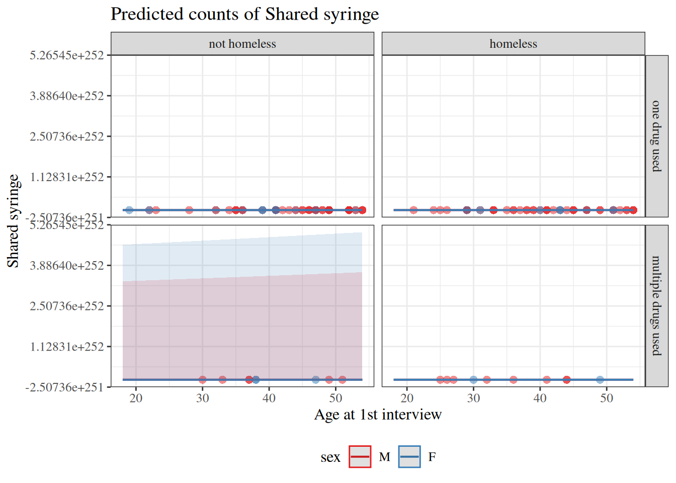
We can still model \(\mu\) as a function of \(X\) and \(T\) as before, and we can combine this model with zero-inflation (as the conditional distribution for the non-zero component).
8.1.1 Example: needle-sharing
Show R code
library(MASS)#need this for glm.nb()glm1.nb=glm.nb( data =needles,shared_syr~age+sex+homeless*polydrug)equatiomatic::extract_eq(glm1.nb)
Table 7: Poisson versus Negative Binomial Regression coefficient estimates
zero-inflation
Show R code
library(glmmTMB)zinf_fit1=glmmTMB( family ="poisson", data =needles, formula =shared_syr~age+sex+homeless*polydrug, ziformula =~age+sex+homeless+polydrug# fit won't converge with interaction)zinf_fit1|>parameters(exponentiate =TRUE)|>print_md()
Another R package for zero-inflated models is pscl (Zeileis et al. (2008)).
zero-inflated negative binomial model
Show R code
library(glmmTMB)zinf_fit1=glmmTMB( family =nbinom2, data =needles, formula =shared_syr~age+sex+homeless*polydrug, ziformula =~age+sex+homeless+polydrug# fit won't converge with interaction)zinf_fit1|>parameters(exponentiate =TRUE)|>print_md()
An alternative to Negative binomial is the “quasipoisson” distribution. I’ve never used it, but it seems to be a method-of-moments type approach rather than maximum likelihood. It models the variance as \(\text{Var}{\left(Y\right)} = \mu\theta\), and estimates \(\theta\) accordingly.
The first equation says \(\sum_i y_i = \sum_i \hat\mu_i\): the total fitted count equals the total observed count.
The second equation says \(\sum_i x_i y_i = \sum_i x_i \hat\mu_i\): the fitted counts are balanced against observed counts, weighted by \(x_i\).
More generally, these score equations say that the residuals \((y_i - \hat\mu_i)\) are orthogonal to each predictor column. This is the GLM analogue of the OLS normal equations.
References
Dobson, Annette J, and Adrian G Barnett. 2018. An Introduction to Generalized Linear Models. 4th ed. CRC press. https://doi.org/10.1201/9781315182780.
Vittinghoff, Eric, David V Glidden, Stephen C Shiboski, and Charles E McCulloch. 2012. Regression Methods in Biostatistics: Linear, Logistic, Survival, and Repeated Measures Models. 2nd ed. Springer. https://doi.org/10.1007/978-1-4614-1353-0.
Zeileis, Achim, Christian Kleiber, and Simon Jackman. 2008. “Regression Models for Count Data in R.”Journal of Statistical Software 27 (8). https://www.jstatsoft.org/v27/i08/.
---title: "Models for Count Outcomes"subtitle: "Poisson regression and variations"format: html: default revealjs: output-file: count-regression-slides.html pdf: output-file: count-regression-handout.pdf docx: output-file: count-regression-handout.docx---# Acknowledgements {.unnumbered}This content is adapted from:- @dobson4e, Chapter 9- @vittinghoff2e, Chapter 8---{{< include shared-config.qmd >}}# Introduction{{< include _subfiles/count-regression/_sec_pois-reg_intro.qmd >}}# Interpreting Poisson regression models {.smaller}{{< include _subfiles/count-regression/_sec_poisson_RRs.qmd >}}# Example: needle-sharing(adapted from @vittinghoff2e, §8)---{{< include exr-needle-sharing.qmd >}}# Inference for count regression models{{< include _subfiles/count-regression/_sec_poisson_inference.qmd >}}# Prediction{{< include _subfiles/count-regression/_sec_pois-reg-preds.qmd >}}# Diagnostics{{< include _subfiles/count-regression/_sec_poisson_dx.qmd >}}---{{< include _subfiles/count-regression/_exm-needle-sharing-dx.qmd >}}# Zero-inflation{{< include _subfiles/count-regression/_sec_zero-inflation.qmd >}}# Over-dispersion{{< include _subfiles/count-regression/_sec-overdispersion.qmd >}}---{{< include _subfiles/count-regression/_note_glm-naming.qmd >}}---## Negative binomial models::: notesThere are alternatives to the Poisson model.Most notably, the [negative binomial model](probability.qmd#sec-nb-dist).We can still model $\mu$ as a function of $X$ and $T$ as before, and we can combine this model with zero-inflation (as the conditional distribution for the non-zero component).:::---### Example: needle-sharing{{< include exr-needle-sharing-extensions.qmd >}}## QuasipoissonAn alternative to Negative binomial is the "quasipoisson" distribution. I've never used it, but it seems to be a method-of-moments type approach rather than maximum likelihood. It models the variance as $\Var{Y} = \mu\theta$, and estimates $\theta$ accordingly.See `?quasipoisson` in R for more.# More on count regression- <https://bookdown.org/roback/bookdown-BeyondMLR/ch-poissonreg.html># Exercises {.unnumbered}{{< include _subfiles/count-regression/_exr-prac-glm-interp.qmd >}}---{{< include _subfiles/count-regression/_exr-prac-glm-score.qmd >}}# References {.unnumbered}::: {#refs}:::