8  Parametric survival models

---

---

Configuring R

Functions from these packages will be used throughout this document:

library(conflicted) # check for conflicting function definitions
# library(printr) # inserts help-file output into markdown output
library(rmarkdown) # Convert R Markdown documents into a variety of formats.
library(pander) # format tables for markdown
library(ggplot2) # graphics
library(ggfortify) # help with graphics
library(dplyr) # manipulate data
library(tibble) # `tibble`s extend `data.frame`s
library(magrittr) # `%>%` and other additional piping tools
library(haven) # import Stata files
library(knitr) # format R output for markdown
library(tidyr) # Tools to help to create tidy data
library(plotly) # interactive graphics
library(dobson) # datasets from Dobson and Barnett 2018
library(parameters) # format model output tables for markdown
library(haven) # import Stata files
library(latex2exp) # use LaTeX in R code (for figures and tables)
library(fs) # filesystem path manipulations
library(survival) # survival analysis
library(survminer) # survival analysis graphics
library(KMsurv) # datasets from Klein and Moeschberger
library(parameters) # format model output tables for
library(webshot2) # convert interactive content to static for pdf
library(forcats) # functions for categorical variables ("factors")
library(stringr) # functions for dealing with strings
library(lubridate) # functions for dealing with dates and times

Here are some R settings I use in this document:

rm(list = ls()) # delete any data that's already loaded into R

conflicts_prefer(dplyr::filter)
ggplot2::theme_set(
  ggplot2::theme_bw() + 
        # ggplot2::labs(col = "") +
    ggplot2::theme(
      legend.position = "bottom",
      text = ggplot2::element_text(size = 12, family = "serif")))

knitr::opts_chunk$set(message = FALSE)
options('digits' = 6)

panderOptions("big.mark", ",")
pander::panderOptions("table.emphasize.rownames", FALSE)
pander::panderOptions("table.split.table", Inf)
conflicts_prefer(dplyr::filter) # use the `filter()` function from dplyr() by default
legend_text_size = 9
run_graphs = TRUE

8.1 Parametric Survival Models

8.1.1 Exponential Distribution

• The exponential distribution is the basic distribution for survival analysis.

\[ \begin{aligned} f(t) &= \lambda e^{-\lambda t}\\ \log{f(t)} &= \log{\lambda}-\lambda t\\ F(t) &= 1-e^{-\lambda t}\\ \text{S}(t)&= e^{-\lambda t}\\ {\Lambda}(t) &= -\log{\text{S}(t)} \\ &= \lambda t\\ {\lambda}(t) &= \lambda\\ \text{E}(T) &= \lambda^{-1} \end{aligned} \]

8.1.2 Weibull Distribution

Using the Kalbfleisch and Prentice (2002) notation:

\[ \begin{aligned} f(t)&= \lambda p (\lambda t)^{p-1}e^{-(\lambda t)^p}\\ F(t)&=1 - e^{-(\lambda t)^p}\\ \text{S}(t)&=e^{-(\lambda t)^p}\\ {\lambda}(t)&=\lambda p (\lambda t)^{p-1}\\ {\Lambda}(t)&=(\lambda t)^p\\ \log{{\Lambda}(t)} &= p \log{\lambda t} \\ &= p \log{\lambda} + p \log{t} \\ \text{E}(T) &= \lambda^{-1} \cdot \Gamma\left(1 + \frac{1}{p}\right) \end{aligned} \]

Note

Recall from calculus:

• \(\Gamma(t) \stackrel{\text{def}}{=}\int_{u=0}^{\infty}u^{t-1}e^{-u}du\)

• \(\Gamma(t) = (t-1)!\) for integers \(t \in \mathbb Z\)

• It is implemented by the gamma() function in R.

Here are some Weibull density functions, with \(\lambda = 1\) and \(p\) varying:

library(ggplot2)
lambda = 1
ggplot() +
  geom_function(
    aes(col = "0.25"),
    fun = \(x) dweibull(x, shape = 0.25, scale = 1/lambda)) +
  geom_function(
    aes(col = "0.5"),
    fun = \(x) dweibull(x, shape = 0.5, scale = 1/lambda)) +
  geom_function(
    aes(col = "1"),
    fun = \(x) dweibull(x, shape = 1, scale = 1/lambda)) +
  geom_function(
    aes(col = "1.5"),
    fun = \(x) dweibull(x, shape = 1.5, scale = 1/lambda)) +
  geom_function(
    aes(col = "2"),
    fun = \(x) dweibull(x, shape = 2, scale = 1/lambda)) +
  geom_function(
    aes(col = "5"),
    fun = \(x) dweibull(x, shape = 5, scale = 1/lambda)) +
  theme_bw() + 
  xlim(0, 2.5) +
  ylab("f(t)") +
  theme(axis.title.y = element_text(angle=0)) +
  theme(legend.position="bottom") +
  guides(
    col = 
      guide_legend(
        title = "p",
        label.theme = 
          element_text(
            size = 12)))

Density functions for Weibull distribution

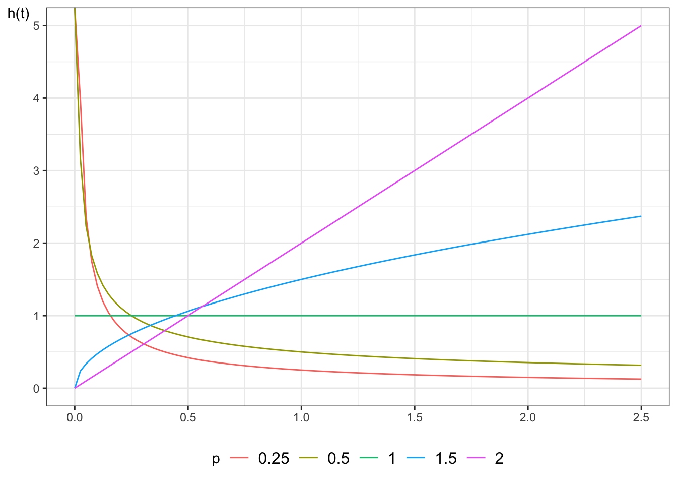
Properties of Weibull hazard functions

Theorem 8.1 If \(T\) has a Weibull distribution, then:

• When \(p=1\), the Weibull distribution simplifies to the exponential distribution
• When \(p > 1\), the hazard is increasing: \(h'(t) > 0\)
• When \(p < 1\), the hazard is decreasing: \(h'(t) < 0\)
• \(\log{{\Lambda}(t)}\) is a straight line relative to \(\log{t}\): \(\log{{\Lambda}(t)} = p \log{\lambda} + p \log{t}\)

---

Exercise 8.1 Prove Theorem 8.1.

---

The Weibull distribution provides more flexibility than the exponential. Figure 8.1 shows some Weibull hazard functions, with \(\lambda = 1\) and \(p\) varying:

library(ggplot2)
library(eha)
lambda = 1

ggplot() +
  geom_function(
    aes(col = "0.25"),
    fun = \(x) hweibull(x, shape = 0.25, scale = 1/lambda)) +
  geom_function(
    aes(col = "0.5"),
    fun = \(x) hweibull(x, shape = 0.5, scale = 1/lambda)) +
  geom_function(
    aes(col = "1"),
    fun = \(x) hweibull(x, shape = 1, scale = 1/lambda)) +
  geom_function(
    aes(col = "1.5"),
    fun = \(x) hweibull(x, shape = 1.5, scale = 1/lambda)) +
  geom_function(
    aes(col = "2"),
    fun = \(x) hweibull(x, shape = 2, scale = 1/lambda)) +
  theme_bw() + 
  xlim(0, 2.5) + 
  ylab(expr(lambda)) +
  theme(axis.title.y = element_text(angle=0)) +
  theme(legend.position="bottom") +
  guides(
    col = 
      guide_legend(
        title = "p",
        label.theme = 
          element_text(
            size = 12)))

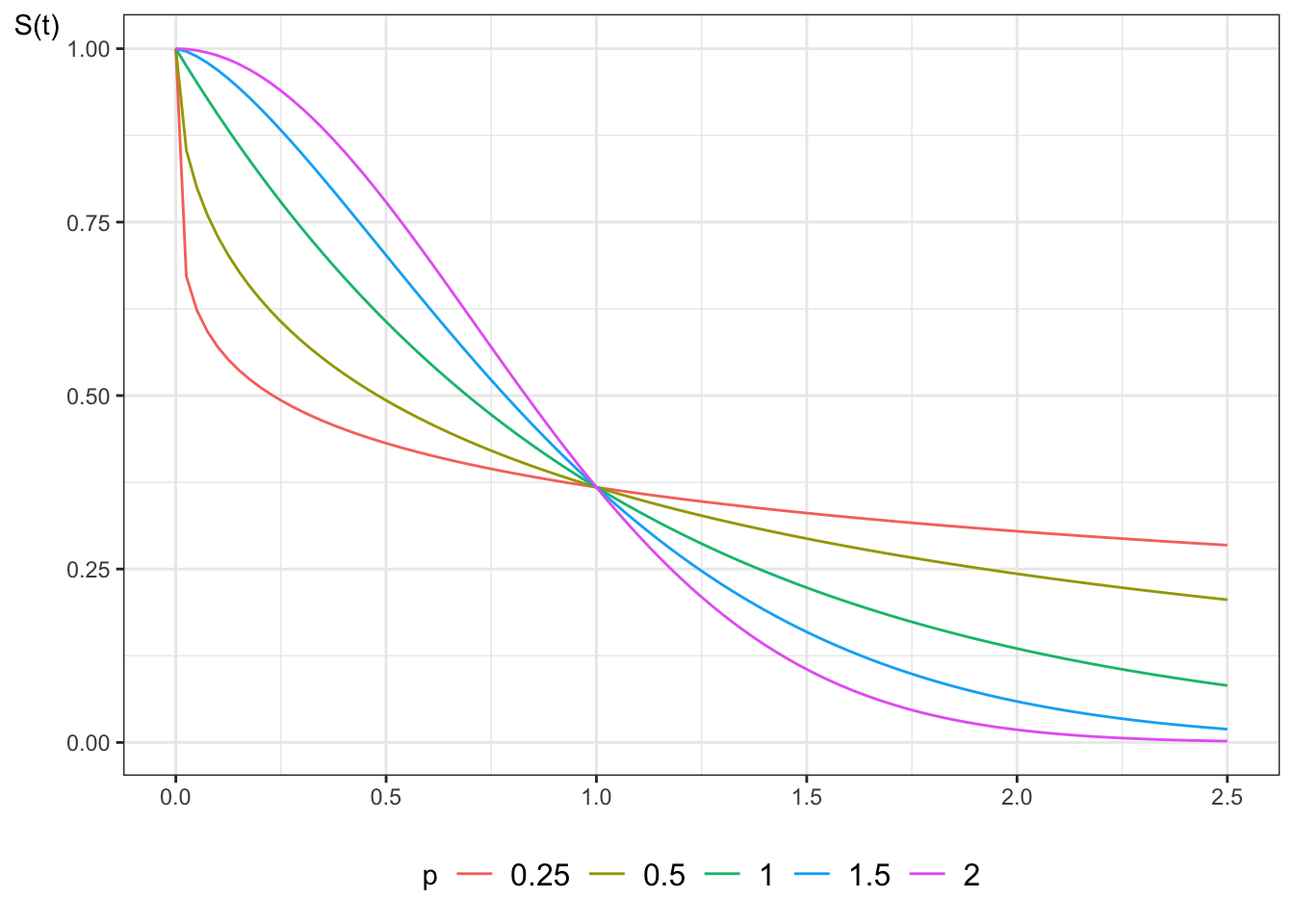
Figure 8.1: Hazard functions for Weibull distribution

---

library(ggplot2)
lambda = 1

ggplot() +
  geom_function(
    aes(col = "0.25"),
    fun = \(x) pweibull(lower = FALSE, x, shape = 0.25, scale = 1/lambda)) +
  geom_function(
    aes(col = "0.5"),
    fun = \(x) pweibull(lower = FALSE, x, shape = 0.5, scale = 1/lambda)) +
  geom_function(
    aes(col = "1"),
    fun = \(x) pweibull(lower = FALSE, x, shape = 1, scale = 1/lambda)) +
  geom_function(
    aes(col = "1.5"),
    fun = \(x) pweibull(lower = FALSE, x, shape = 1.5, scale = 1/lambda)) +
  geom_function(
    aes(col = "2"),
    fun = \(x) pweibull(lower = FALSE, x, shape = 2, scale = 1/lambda)) +
  theme_bw() + 
  xlim(0, 2.5) + 
  ylab("S(t)") +
  theme(axis.title.y = element_text(angle=0)) +
  theme(legend.position="bottom") +
  guides(
    col = 
      guide_legend(
        title = "p",
        label.theme = 
          element_text(
            size = 12)))

Figure 8.2: Survival functions for Weibull distribution

8.1.3 Exponential Regression

For each subject \(i\), define a linear predictor:

\[ \begin{aligned} \eta(\tilde{x}) &= \beta_0 + (\beta_1x_1 + \dots + \beta_p x_p)\\ {\lambda}(t|\tilde{x}) &= \text{exp}{\left\{\eta(\tilde{x})\right\}}\\ {\lambda}_0 &\stackrel{\text{def}}{=} {\lambda}(t|\tilde{0})\\ &= \text{exp}{\left\{\eta(\tilde{0})\right\}}\\ &= \text{exp}{\left\{\beta_0 + (\beta_1 \cdot 0 + \dots + \beta_p \cdot 0)\right\}}\\ &= \text{exp}{\left\{\beta_0 + 0\right\}}\\ &= \text{exp}{\left\{\beta_0\right\}}\\ \end{aligned} \]

We let the linear predictor have a constant term, and when there are no additional predictors the hazard is \(\lambda = \text{exp}{\left\{\beta_0\right\}}\). This has a log link as in a generalized linear model. Since the hazard does not depend on \(t\), the hazards are (trivially) proportional.

8.1.4 Accelerated Failure Time

Previously, we assumed the hazards were proportional; that is, the covariates multiplied the baseline hazard function:

\[ \begin{aligned} h(T=t|X=x) &\stackrel{\text{def}}{=} p(T=t|X=x,T \ge t)\\ &= {\lambda}(t|X=0)\cdot \text{exp}{\left\{\eta(x)\right\}}\\ &= {\lambda}(t|X=0)\cdot \theta(x)\\ &= {\lambda}_0(t)\cdot \theta(x) \end{aligned} \]

and correspondingly,

\[ \begin{aligned} {\Lambda}(t|x) &= \theta(x){\Lambda}_0(t)\\ \text{S}(t|x) &= \text{exp}{\left\{-{\Lambda}(t|x)\right\}}\\ &= \text{exp}{\left\{-\theta(x)\cdot {\Lambda}_0(t)\right\}}\\ &= {\left(\text{exp}{\left\{- {\Lambda}_0(t)\right\}}\right)}^{\theta(x)}\\ &= {\left(\text{S}_0(t)\right)}^{\theta(x)}\\ \end{aligned} \]

An alternative modeling assumption would be \[\text{S}(t|X=x)=\text{S}_0(t\cdot \theta(x))\] where \(\theta(x)=\text{exp}{\left\{\eta(x)\right\}}\), \(\eta(x) =\beta_1x_1+\cdots+\beta_px_p\), and \(\text{S}_0(t)=\text{P}(T\ge t|X=0)\) is the base survival function.

Then

\[ \begin{aligned} \text{E}[T|X=x] &= \int_{t=0}^{\infty} \text{S}(t|x)dt\\ &= \int_{t=0}^{\infty} \text{S}_0(t\cdot \theta(x))dt\\ &= \int_{u=0}^{\infty} \text{S}_0(u)du \cdot \theta(x)^{-1}\\ &= \theta(x)^{-1} \cdot \int_{u=0}^{\infty} \text{S}_0(u)du\\ &= \theta(x)^{-1} \cdot \text{E}[T|X=0]\\ \end{aligned} \] So the mean of \(T\) given \(X=x\) is the baseline mean divided by \(\theta(x) = \text{exp}{\left\{\eta(x)\right\}}\).

This modeling strategy is called an accelerated failure time model, because covariates cause uniform acceleration (or slowing) of failure times.

Additionally:

\[ \begin{aligned} {\Lambda}(t|x) &= {\Lambda}_0(\theta(x)\cdot t)\\ {\lambda}(t|x) &= \theta(x) \cdot {\lambda}_0(\theta(x)\cdot t) \end{aligned} \]

If the base distribution is exponential with parameter \(\lambda\) then

\[ \begin{aligned} \text{S}(t|x) &= \text{exp}{\left\{-\lambda \cdot t \theta(x)\right\}}\\ &= [\text{exp}{\left\{-\lambda t\right\}}]^{\theta(x)}\\ \end{aligned} \]

which is an exponential model with base hazard multiplied by \(\theta(x)\), which is also the proportional hazards model.

In terms of the log survival time \(Y=\log{T}\) the model can be written as

\[ \begin{aligned} Y&=\alpha-\eta+W\\ \alpha&= -\log{\lambda} \end{aligned} \]

where \(W\) has the extreme value distribution. The estimated parameter \(\lambda\) is the intercept and the other coefficients are those of \(\eta\), which will be the opposite sign of those for coxph.

For a Weibull distribution, the hazard function and the survival function are

\[ \begin{aligned} {\lambda}(t)&=\lambda p (\lambda t)^{p-1}\\ \text{S}(t)&=e^{-(\lambda t)^p} \end{aligned} \]

We can construct a proportional hazards model by using a linear predictor \(\eta_i\) without constant term and letting \(\theta_i=e^{\eta_i}\) we have

\[ \begin{aligned} {\lambda}(t)&=\lambda p (\lambda t)^{p-1}\theta_i \end{aligned} \]

A distribution with \({\lambda}(t)=\lambda p (\lambda t)^{p-1}\theta_i\) is a Weibull distribution with parameters \(\lambda^*=\lambda \theta_i^{1/p}\) and \(p\) so the survival function is

\[ \begin{aligned} S^*(t)&=e^{-(\lambda^* t)^p}\\ &=e^{-(\lambda \theta^{1/p} t)^p}\\ &= \text{S}(t\theta^{1/p}) \end{aligned} \]

so this is also an accelerated failure time model.

In terms of the log survival time \(Y=\log{T}\) the model can be written as

\[ \begin{aligned} Y&=\alpha-\sigma\eta+\sigma W\\ \alpha&= -\log{\lambda}\\ \sigma &= 1/p \end{aligned} \]

where \(W\) has the extreme value distribution. The estimated parameter \(\lambda\) is the intercept and the other coefficients are those of \(\eta\), which will be the opposite sign of those for coxph.

These AFT models are log-linear, meaning that the linear predictor has a log link. The exponential and the Weibull are the only log-linear models that are simultaneously proportional hazards models. Other parametric distributions can be used for survival regression either as a proportional hazards model or as an accelerated failure time model.

8.1.5 Dataset: Leukemia treatments

Remission survival times on 42 leukemia patients, half on new treatment, half on standard treatment.

This is the same data as the drug6mp data from KMsurv, but with two other variables and without the pairing.

library(haven)
library(survival)
anderson = 
  paste0(
    "http://web1.sph.emory.edu/dkleinb/allDatasets",
    "/surv2datasets/anderson.dta") |> 
  read_dta() |> 
  mutate(
    status = status |> 
      case_match(
        1 ~ "relapse",
        0 ~ "censored"
      ),
    sex = sex |> 
      case_match(
        0 ~ "female",
        1 ~ "male"
      ),
    
    rx = rx |> 
      case_match(
        0 ~ "new",
        1 ~ "standard"
      ),
    
    surv = Surv(time = survt,event = (status == "relapse"))
  ) 

print(anderson)

Cox semi-parametric model

anderson.cox0 = coxph(
  formula = surv ~ rx,
  data = anderson)
summary(anderson.cox0)
#> Call:
#> coxph(formula = surv ~ rx, data = anderson)
#> 
#>   n= 42, number of events= 30 
#> 
#>             coef exp(coef) se(coef)    z Pr(>|z|)    
#> rxstandard 1.572     4.817    0.412 3.81  0.00014 ***
#> ---
#> Signif. codes:  0 '***' 0.001 '**' 0.01 '*' 0.05 '.' 0.1 ' ' 1
#> 
#>            exp(coef) exp(-coef) lower .95 upper .95
#> rxstandard      4.82      0.208      2.15      10.8
#> 
#> Concordance= 0.69  (se = 0.041 )
#> Likelihood ratio test= 16.4  on 1 df,   p=5e-05
#> Wald test            = 14.5  on 1 df,   p=1e-04
#> Score (logrank) test = 17.2  on 1 df,   p=3e-05

Weibull parametric model

anderson.weib <- survreg(
  formula = surv ~ rx,
  data = anderson,
  dist = "weibull")
summary(anderson.weib)
#> 
#> Call:
#> survreg(formula = surv ~ rx, data = anderson, dist = "weibull")
#>              Value Std. Error     z       p
#> (Intercept)  3.516      0.252 13.96 < 2e-16
#> rxstandard  -1.267      0.311 -4.08 4.5e-05
#> Log(scale)  -0.312      0.147 -2.12   0.034
#> 
#> Scale= 0.732 
#> 
#> Weibull distribution
#> Loglik(model)= -106.6   Loglik(intercept only)= -116.4
#>  Chisq= 19.65 on 1 degrees of freedom, p= 9.3e-06 
#> Number of Newton-Raphson Iterations: 5 
#> n= 42

Exponential parametric model

anderson.exp <- survreg(
  formula = surv ~ rx,
  data = anderson,
  dist = "exp")
summary(anderson.exp)
#> 
#> Call:
#> survreg(formula = surv ~ rx, data = anderson, dist = "exp")
#>              Value Std. Error     z       p
#> (Intercept)  3.686      0.333 11.06 < 2e-16
#> rxstandard  -1.527      0.398 -3.83 0.00013
#> 
#> Scale fixed at 1 
#> 
#> Exponential distribution
#> Loglik(model)= -108.5   Loglik(intercept only)= -116.8
#>  Chisq= 16.49 on 1 degrees of freedom, p= 4.9e-05 
#> Number of Newton-Raphson Iterations: 4 
#> n= 42

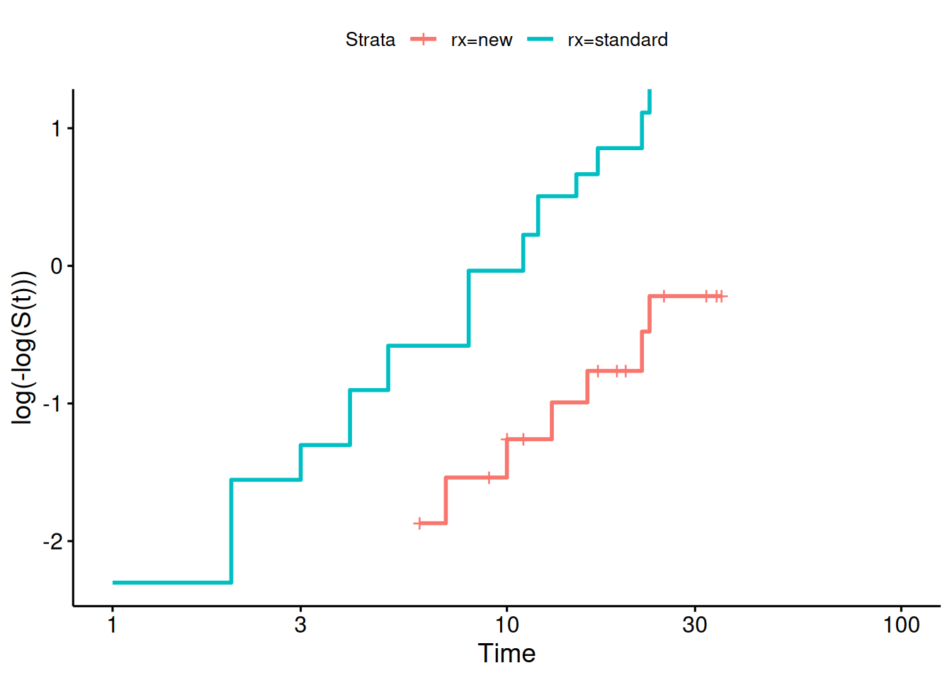
Diagnostic - complementary log-log survival plot

library(survminer)
survfit(
  formula = surv ~ rx,
  data = anderson) |> 
  ggsurvplot(fun = "cloglog")

If the cloglog plot is linear, then a Weibull model may be ok.

8.2 Combining left-truncation and interval-censoring

From [https://stat.ethz.ch/pipermail/r-help/2015-August/431733.html]:

coxph does left truncation but not left (or interval) censoring survreg does interval censoring but not left truncation (or time dependent covariates).

• Terry Therneau, August 31, 2015