Welcome to Epidemiology 204: Quantitative Epidemiology III (Statistical Models).
In this course, we will start where Epi 203 left off: with linear regression models.
Note
Epi 203/STA 130B/STA 131B is a prerequisite for this course. If you haven’t passed one of these courses, please talk to me ASAP.
1.1.1 What you should already know
Epi 202: probability models for different data types
Probability distributions
binomial
Poisson
Gaussian
exponential
Characteristics of probability distributions
Mean, median, mode, quantiles
Variance, standard deviation, overdispersion
Characteristics of samples
independence, dependence, covariance, correlation
ranks, order statistics
identical vs nonidentical distribution (homogeneity vs heterogeneity)
Laws of Large Numbers
Central Limit Theorem for the mean of an iid sample
Epi 203: inference for one or several homogenous populations
the maximum likelihood inference framework:
likelihood functions
log-likelihood functions
score functions
estimating equations
information matrices
point estimates
standard errors
confidence intervals
hypothesis tests
p-values
Hypothesis tests for one, two, and >2 groups:
t-tests/ANOVA for Gaussian models
chi-square tests for binomial and Poisson models
nonparametric tests:
Wilcoxon signed-rank test for matched pairs
Mann–Whitney/Kruskal-Wallis rank sum test for ≥2 independent samples
Fisher’s exact test for contingency tables
Cochran–Mantel–Haenszel-Cox log-rank test
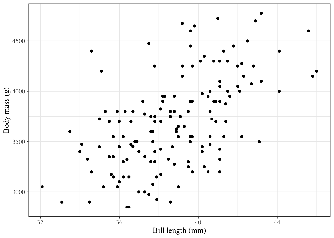
Some linear regression
For all of the quantities above, and especially for confidence intervals and p-values, you should know how both: - how to compute them - how to interpret them
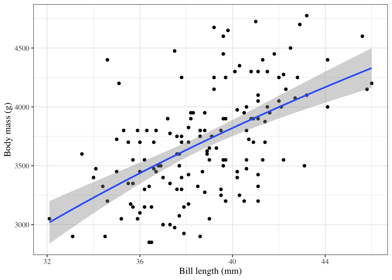
ggpenguins=palmerpenguins::penguins|>ggplot(aes(x =bill_length_mm , y =body_mass_g, color =species))+geom_point()+stat_smooth( method ="lm", formula =y~x, geom ="smooth")+xlab("Bill length (mm)")+ylab("Body mass (g)")ggpenguins|>print()
Wickham, Hadley, Mine Çetinkaya-Rundel, and Garrett Grolemund. 2023. R for Data Science. " O’Reilly Media, Inc.". https://r4ds.hadley.nz/.
Source Code
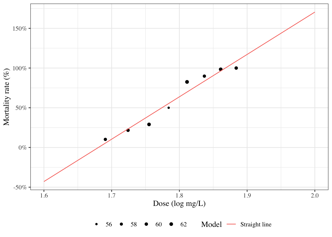
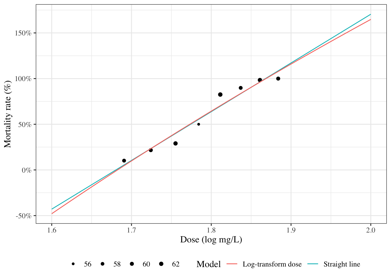
# Introduction---{{< include shared-config.qmd >}}## Introduction to Epi 204 {.scrollable}Welcome to Epidemiology 204: Quantitative Epidemiology III (Statistical Models).In this course, we will start where Epi 203 left off: with linear regression models.::: callout-noteEpi 203/STA 130B/STA 131B is a prerequisite for this course. If you haven't passed one of these courses, please talk to me ASAP.:::### What you should already know {.scrollable}{{< include prereq-knowledge.qmd >}}### What we will cover in this course* Linear (Gaussian) regression models (review and more details)* Regression models for non-Gaussian outcomes + binary + count + time to event* Statistical analysis using R## Regression modelsWhy do we need them?* continuous predictors* not enough data to analyze some subgroups individually### Example: Adelie penguins```{r}#| label: fig-palmer-1#| fig-cap: Palmer penguins#| echo: falselibrary(ggplot2)library(plotly)library(dplyr)ggpenguins <- palmerpenguins::penguins |> dplyr::filter(species =="Adelie") |>ggplot(aes(x = bill_length_mm , y = body_mass_g)) +geom_point() +xlab("Bill length (mm)") +ylab("Body mass (g)")print(ggpenguins)```### Linear regression```{r}#| label: fig-palmer-2#| fig-cap: Palmer penguins with linear regression fitggpenguins2 = ggpenguins +stat_smooth(method ="lm",formula = y ~ x,geom ="smooth")ggpenguins2 |>print()```### Curved regression lines```{r}#| label: fig-palmer-3#| fig-cap: Palmer penguins - curved regression linesggpenguins2 = ggpenguins +stat_smooth(method ="lm",formula = y ~log(x),geom ="smooth") +xlab("Bill length (mm)") +ylab("Body mass (g)")ggpenguins2```### Multiple regression```{r}#| label: fig-palmer-4#| fig-cap: "Palmer penguins - multiple groups"ggpenguins = palmerpenguins::penguins |>ggplot(aes(x = bill_length_mm , y = body_mass_g,color = species ) ) +geom_point() +stat_smooth(method ="lm",formula = y ~ x,geom ="smooth") +xlab("Bill length (mm)") +ylab("Body mass (g)")ggpenguins |>print()```### Modeling non-Gaussian outcomes```{r}#| label: fig-beetles_1a#| fig-cap: "Mortality rates of adult flour beetles after five hours' exposure to gaseous carbon disulphide (Bliss 1935)"library(glmx)data(BeetleMortality)beetles = BeetleMortality |>mutate(pct = died/n,survived = n - died )plot1 = beetles |>ggplot(aes(x = dose, y = pct)) +geom_point(aes(size = n)) +xlab("Dose (log mg/L)") +ylab("Mortality rate (%)") +scale_y_continuous(labels = scales::percent) +# xlab(bquote(log[10]), bquote(CS[2])) +scale_size(range =c(1,2))print(plot1)```### Why don't we use linear regression?```{r}#| label: fig-beetles-plot1#| fig-cap: "Mortality rates of adult flour beetles after five hours' exposure to gaseous carbon disulphide (Bliss 1935)"beetles_long = beetles |>reframe(.by =everything(),outcome =c(rep(1, times = died), rep(0, times = survived)) )lm1 = beetles_long |>lm(formula = outcome ~ dose, data = _)range1 =range(beetles$dose) +c(-.2, .2)f.linear =function(x) predict(lm1, newdata =data.frame(dose = x))plot2 = plot1 +geom_function(fun = f.linear, aes(col ="Straight line")) +labs(colour="Model", size ="")print(plot2)```### Zoom out```{r}#| label: fig-beetles2#| fig-cap: Mortality rates of adult flour beetles after five hours' exposure to gaseous carbon disulphide (Bliss 1935)#| echo: falseprint(plot2 +expand_limits(x =c(1.6, 2)))```### log transformation of dose?```{r}#| label: fig-beetles3#| fig-cap: Mortality rates of adult flour beetles after five hours' exposure to gaseous carbon disulphide (Bliss 1935)lm2 = beetles_long |>lm(formula = outcome ~log(dose), data = _)f.linearlog =function(x) predict(lm2, newdata =data.frame(dose = x))plot3 = plot2 +expand_limits(x =c(1.6, 2)) +geom_function(fun = f.linearlog, aes(col ="Log-transform dose"))print(plot3 +expand_limits(x =c(1.6, 2)))```### Logistic regression```{r}#| label: fig-beetles4b#| fig-cap: Mortality rates of adult flour beetles after five hours' exposure to gaseous carbon disulphide (Bliss 1935)glm1 = beetles |>glm(formula =cbind(died, survived) ~ dose, family ="binomial")f =function(x) predict(glm1, newdata =data.frame(dose = x), type ="response")plot4 = plot3 +geom_function(fun = f, aes(col ="Logistic regression"))print(plot4)```### Three parts to regression models- What distribution does the outcome have for a specific sub-population defined by covariates? (**outcome model**)- How does the combination of covariates relate to the mean? (**link function**)- How do the covariates combine? (**linear predictor/linear component**)$$\eta \eqdef \vx \' \vb = \b_0 + \b_1 x_1 + \b_2 x_2 + ...$$