---
title: "Probability"
format:
html: default
revealjs:
output-file: probability-slides.html
pdf:
output-file: probability-handout.pdf
docx:
output-file: probability-handout.docx
---
{{< include shared-config.qmd >}}
---
Most of the content in this chapter should be review from UC Davis Epi 202.
# Core properties of probabilities
## Defining probabilities
::: {#def-probability}
#### Probability measure
A **probability measure**, often denoted $\Pr()$ or $\P()$,
is a function whose domain is a
[$\sigma$-algebra](https://en.wikipedia.org/wiki/%CE%A3-algebra)
of possible outcomes, $\mathscr{S}$,
and which satisfies the following properties:
1. For any statistical event $A \in \mathscr{S}$, $\Pr(A) \ge 0$.
2. The probability of the union of all outcomes ($\Omega \eqdef \cup \mathscr{S}$)
is 1:
$$\Pr(\Omega) = 1$$
3. The probability of the union of countably many mutually disjoint events
$A_1, A_2, \ldots$ (where $A_i \cap A_j = \emptyset$ for all $i \neq j$)
is equal to the sum of their probabilities
(*countable additivity* or *sigma-additivity*):
$$\Pr\!\left(\bigcup_{i=1}^{\infty} A_i\right) = \sum_{i=1}^{\infty} \Pr(A_i)$$
:::
::: notes
Property 3 (*countable additivity*) is stronger than *finite additivity*,
which only requires
$$\Pr(A_1 \cup \cdots \cup A_n) = \sum_{i=1}^{n} \Pr(A_i)$$
for every finite collection of mutually disjoint events.
Countable additivity implies finite additivity
(set $A_{n+1} = A_{n+2} = \cdots = \emptyset$ in property 3,
using $\Pr(\emptyset) = 0$),
but not vice versa:
there exist set functions that satisfy finite additivity
but fail countable additivity
(see [Wikipedia: Sigma-additive set function — An additive function which is not σ-additive](https://en.wikipedia.org/wiki/Sigma-additive_set_function#An_additive_function_which_is_not_%CF%83-additive)).
Requiring countable additivity enables results such as
the continuity of probability
(if $A_1 \supseteq A_2 \supseteq \cdots$ with $\bigcap_i A_i = \emptyset$,
then $\Pr(A_i) \to 0$)
and underpins the @thm-total-prob for countable partitions.
:::
---
:::{#thm-prob-subset}
#### Probability of a subset's intersection
If $A$ and $B$ are statistical events and $A\subseteq B$, then $\Pr(A \cap B) = \Pr(A)$.
:::
---
::: proof
Left to the reader for now.
:::
---
:::{#thm-total-prob-1}
#### An event and its complement sum to 1
$$\Pr(A) + \Pr(\neg A) = 1$$
:::
---
::: proof
By properties 2 and 3 of @def-probability.
:::
---
:::{#cor-p-neg0}
#### Complement rule
$$\Pr(\neg A) = 1 - \Pr(A)$$
:::
---
::: proof
By @thm-total-prob-1 and algebra.
:::
---
:::{#cor-p-neg}
#### Complement rule in probability ($\pi$) notation
If the probability of an outcome $A$ is $\Pr(A)=\pi$,
then the probability that $A$ does not occur is:
$$\Pr(\neg A)= 1 - \pi$$
:::
---
::: proof
Using @cor-p-neg0:
$$
\ba
\Pr(\neg A) &= 1 - \Pr(A)
\\ &= 1 - \pi
\ea
$$
:::
---
## Conditional probability
:::{#def-conditional-prob}
### Conditional probability
For two events $A$ and $B$ with $\Pr(B) > 0$,
the **conditional probability** of $A$ given $B$,
denoted $\Pr(A \mid B)$,
is:
$$\Pr(A \mid B) \eqdef \frac{\Pr(A \cap B)}{\Pr(B)}$$
:::
---
:::{#thm-law-conditional-prob}
### Law of conditional probability
For any two events $A$ and $B$ with $\Pr(B) > 0$:
$$\Pr(A \cap B) = \Pr(A \mid B) \cd \Pr(B)$$
:::
---
::: proof
Rearranging @def-conditional-prob:
$$
\ba
\Pr(A \mid B) &= \frac{\Pr(A \cap B)}{\Pr(B)}
\\ \Pr(A \cap B) &= \Pr(A \mid B) \cd \Pr(B)
\ea
$$
:::
---
:::{#exm-law-conditional-prob}
#### Applying the law of conditional probability
Suppose 30% of adults exercise regularly ($\Pr(E) = 0.30$),
and among adults who exercise regularly,
60% have low blood pressure ($\Pr(L \mid E) = 0.60$).
Then the probability that a randomly selected adult both exercises
regularly and has low blood pressure is:
$$
\ba
\Pr(L \cap E) &= \Pr(L \mid E) \cd \Pr(E)
\\&= 0.60 \cd 0.30
\\&= 0.18
\ea
$$
:::
---
:::{#thm-total-prob}
### Law of total probability
If $B_1, B_2, \ldots$ is a countable partition of the sample space
(i.e., countably many mutually exclusive events whose union is the entire sample space),
then for any event $A$:
$$\Pr(A) = \sum_{i=1}^{\infty} \Pr(A \mid B_i) \cd \Pr(B_i)$$
:::
---
::: proof
Since $B_1, B_2, \ldots$ partition the sample space,
the events $A \cap B_1, A \cap B_2, \ldots$ are mutually exclusive and their
union is $A$.
By property 3 of @def-probability (countable additivity),
and then by @thm-law-conditional-prob:
$$
\ba
\Pr(A)
&= \sum_{i=1}^{\infty} \Pr(A \cap B_i)
\\&= \sum_{i=1}^{\infty} \Pr(A \mid B_i) \cd \Pr(B_i)
\ea
$$
:::
---
:::{#thm-bayes}
### Bayes' theorem
For any two events $A$ and $B$ with $\Pr(A) > 0$ and $\Pr(B) > 0$:
$$\Pr(A \mid B) = \frac{\Pr(B \mid A) \cd \Pr(A)}{\Pr(B)}$$
:::
---
::: proof
Apply @def-conditional-prob to both $\Pr(A \mid B)$ and $\Pr(B \mid A)$:
$$
\ba
\Pr(A \mid B)
&= \frac{\Pr(A \cap B)}{\Pr(B)}
\\&= \frac{\Pr(B \mid A) \cd \Pr(A)}{\Pr(B)}
\ea
$$
The second equality follows from @thm-law-conditional-prob applied to $\Pr(B \cap A) = \Pr(B \mid A) \cd \Pr(A)$.
:::
---
:::{#exm-bayes}
#### Positive predictive value of a medical test
Suppose a disease test has 99% sensitivity and 99% specificity,
and the prevalence of the disease in the population is 7%.
Let $D$ be the event "person has the disease"
and $+$ be the event "test is positive".
Then:
- $\Pr(+ \mid D) = 0.99$ (sensitivity)
- $\Pr(\neg + \mid \neg D) = 0.99$ (specificity),
so the false positive rate is $\Pr(+ \mid \neg D) = 1 - 0.99 = 0.01$
- $\Pr(D) = 0.07$ (prevalence)
By Bayes' theorem (@thm-bayes) and the law of total probability (@thm-total-prob):
$$
\ba
\Pr(D \mid +)
&= \frac{\Pr(+ \mid D) \cd \Pr(D)}{\Pr(+)}
\\&= \frac{\Pr(+ \mid D) \cd \Pr(D)}{\Pr(+ \mid D) \cd \Pr(D) + \Pr(+ \mid \neg D) \cd \Pr(\neg D)}
\\&= \frac{0.99 \cd 0.07}{0.99 \cd 0.07 + 0.01 \cd 0.93}
\\&= \frac{0.0693}{0.0693 + 0.0093}
\\&= \frac{0.0693}{0.0786}
\\&\approx 0.88
\ea
$$
Even with a highly accurate test (99% sensitive and 99% specific),
only about 88% of people who test positive actually have the disease,
because the disease prevalence is relatively low (7%).
:::
# Key probability distributions
{{< include _subfiles/probability/_sec_distn_uses.qmd >}}
## The Bernoulli distribution {#sec-bern-dist}
{{< include bernoulli.qmd >}}
---
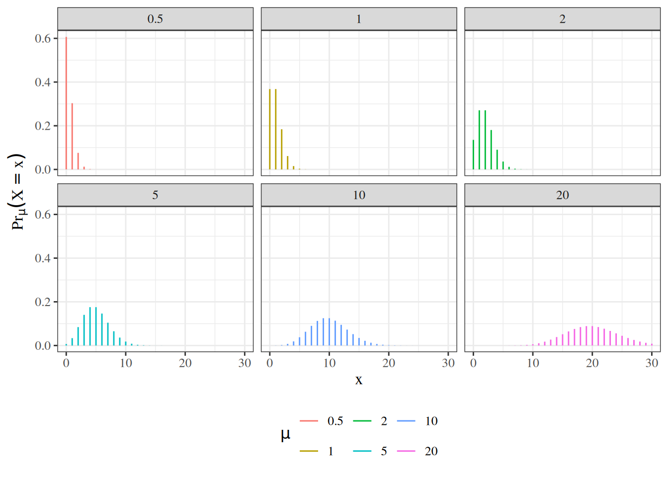
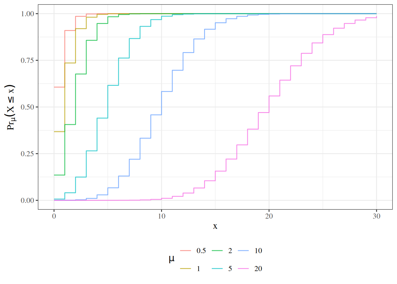
## The Poisson distribution {#sec-poisson-dist}
{{< include poisson.qmd >}}
---
## The Negative-Binomial distribution {#sec-nb-dist}
{{< include negbinom.qmd >}}
## Weibull Distribution {#sec-weibull}
$$
\begin{aligned}
p(t)&= \alpha\lambda x^{\alpha-1}\text{e}^{-\lambda x^\alpha}\\
\haz(t)&=\alpha\lambda x^{\alpha-1}\\
\surv(t)&=\text{e}^{-\lambda x^\alpha}\\
E(T)&= \Gamma(1+1/\alpha)\cdot \lambda^{-1/\alpha}
\end{aligned}
$$
When $\alpha=1$ this is the exponential. When $\alpha>1$ the hazard is
increasing and when $\alpha < 1$ the hazard is decreasing. This provides
more flexibility than the exponential.
We will see more of this distribution later.
# Characteristics of probability distributions
## Probability density function {#sec-prob-dens}
{{< include _subfiles/probability/_def-pdf.qmd >}}
---
:::{#def-cdf}
### Cumulative distribution function (CDF)
For a random variable $X$,
its population CDF is
$$F(t)=\Pr(X\le t), \quad t\in\mathbb{R}.$$
:::
:::{#def-quantile-function}
#### Quantile function (population inverse CDF)
For a random variable $X$
with [cumulative distribution function (CDF)](#def-cdf) $F$,
its population quantile function
(generalized inverse of $F$)
is
$$Q(p)=\inf\{t:F(t)\ge p\}, \quad 0<p\le 1.$$
:::
---
:::{#thm-density-vs-CDF}
## Density function is derivative of CDF
The density function $f(t)$ or $\p(T=t)$ for a random variable $T$ at value $t$ is equal to the derivative of the cumulative probability function $F(t) \eqdef P(T\le t)$; that is:
$$f(t) \eqdef \deriv{t} F(t)$$
:::
---
:::{#thm-density-sums-to-one}
### Density functions integrate to 1
For any density function $f(x)$,
$$\int_{x \in \rangef{X}} f(x) dx = 1$$
:::
---
## Hazard function {#sec-prob-haz}
{{< include _subfiles/shared/_def-hazard.qmd >}}
---
{{< include _subfiles/probability/_sec-survival-dist-fns.qmd >}}
---
{{< include _subfiles/shared/_surv_diagram.qmd >}}
---
## Expectation {#sec-expectation}
:::{#def-expectation}
## Expectation, expected value, population mean \index{expectation} \index{expected value}
The **expectation**, **expected value**, or **population mean** of a *continuous* random variable $X$, denoted $\E{X}$, $\mu(X)$, or $\mu_X$, is the weighted mean of $X$'s possible values, weighted by the probability density function of those values:
$$\E{X} = \int_{x\in \rangef{X}} x \cdot \p(X=x)dx$$
The **expectation**, **expected value**, or **population mean** of a *discrete* random variable $X$,
denoted $\E{X}$, $\mu(X)$, or $\mu_X$,
is the mean of $X$'s possible values,
weighted by the probability mass function of those values:
$$\E{X} = \sum_{x \in \rangef{X}} x \cdot \P(X=x)$$
(c.f. <https://en.wikipedia.org/wiki/Expected_value>)
:::
---
:::{#thm-bernoulli-mean}
### Expectation of the Bernoulli distribution
The expectation of a Bernoulli random variable with parameter $\pi$ is:
$$\E{X} = \pi$$
:::
---
:::{.proof}
$$
\ba
\E{X}
&= \sum_{x\in \rangef{X}} x \cd \P(X=x)
\\&= \sum_{x\in \set{0,1}} x \cd \P(X=x)
\\&= \paren{0 \cd \P(X=0)} + \paren{1 \cd \P(X=1)}
\\&= \paren{0 \cd (1-\pi)} + \paren{1 \cd \pi}
\\&= 0 + \pi
\\&= \pi
\ea
$$
:::
---
{{< include _subfiles/probability/_thm-surv-mean.qmd >}}
::: proof
We prove the continuous case, in which $T$ has a density $\pdf$.
The result follows from applying Tonelli's
theorem (hypothesis (a) of
[Fubini–Tonelli](math-prereqs.qmd#thm-fubini-tonelli)) to the function
$g(t, u) = \pdf(u) \cdot \indicp{0 \le t \le u}$ on the product space
$[0, \infty) \times [0, \infty)$: $g$ is nonnegative everywhere and
vanishes outside the (unbounded) triangular region
$D = \{(t, u) : 0 \le t \le u < \infty\}$, so the iterated integrals
over $D$ are exchangeable.
Since $\pdf(u) \ge 0$, hypothesis (a) of
[Fubini–Tonelli](math-prereqs.qmd#thm-fubini-tonelli)
(the nonnegative case, **Tonelli's theorem**) applies, and we may
exchange the order of integration over $D$:
$$
\ba
\E{T}
&= \int_{u=0}^{\infty} u\,\pdf(u)\,du\\
&= \int_{u=0}^{\infty}\paren{\int_{t=0}^{u} 1\,dt}\pdf(u)\,du\\
&= \int_{u=0}^{\infty}\int_{t=0}^{u} \pdf(u)\,dt\,du\\
&= \int_{t=0}^{\infty}\int_{u=t}^{\infty} \pdf(u)\,du\,dt\\
&= \int_{t=0}^{\infty}\P(T>t)\,dt\\
&= \int_{t=0}^{\infty}\surv(t)\,dt.
\ea
$$
:::
{{< slidebreak >}}
:::{#exm-fubini-survfn}
#### Mean of an exponential random variable via survival function
Let $T \sim \mathrm{Exponential}(\lambda)$, so $\surv(t) = \ef{-\lambda t}$
for $t \ge 0$.
By @thm-surv-mean:
$$
\ba
\E{T}
&= \int_0^\infty \surv(t)\,dt\\
&= \int_0^\infty \ef{-\lambda t}\,dt\\
&= \sb{-\frac{1}{\lambda}\ef{-\lambda t}}_0^\infty\\
&= \frac{1}{\lambda},
\ea
$$
confirming the standard result $\E{T} = 1/\lambda$.
:::
---
:::{#thm-lotus}
### Law of the Unconscious Statistician (LOTUS)
For any function $g$ of a *discrete* random variable $X$:
$$\E{g(X)} = \sum_{x \in \rangef{X}} g(x) \cd \P(X=x)$$
:::
---
::: proof
Let $Y = g(X)$.
By @def-expectation applied to $Y$:
$$
\ba
\E{g(X)}
&= \E{Y}
\\&= \sum_{y \in \rangef{Y}} y \cd \P(Y=y)
\\&= \sum_{y \in \rangef{Y}} y \cd \P(g(X)=y)
\\&= \sum_{y \in \rangef{Y}} y \cd \sum_{\substack{x \in \rangef{X} \\ g(x) = y}} \P(X=x)
\\&= \sum_{x \in \rangef{X}} g(x) \cd \P(X=x)
\ea
$$
where the last equality follows by rearranging the double sum,
grouping each term $x$ by its image $y = g(x)$.
:::
---
::: notes
LOTUS says that to compute $\E{g(X)}$,
we do not need to first find the distribution of $g(X)$;
we can compute the expectation directly using the distribution of $X$.
For a *continuous* random variable $X$ with density $\p(X=x)$,
the analogous formula is:
$$\E{g(X)} = \int_{x \in \rangef{X}} g(x) \cd \p(X=x)\, dx$$
:::
---
:::{#exm-lotus}
#### Expected value of $X^2$ for a Bernoulli variable
Let $X \sim \Ber(\pi)$.
By LOTUS (@thm-lotus):
$$
\ba
\E{X^2}
&= \sum_{x \in \set{0,1}} x^2 \cd \P(X=x)
\\&= 0^2 \cd \P(X=0) + 1^2 \cd \P(X=1)
\\&= 0^2 \cd (1-\pi) + 1^2 \cd \pi
\\&= 0 + \pi
\\&= \pi
\ea
$$
:::
---
:::{#def-cond-expectation}
### Conditional expectation
**Discrete case.**
Let $X$ and $Y$ be jointly distributed discrete random variables.
The **conditional probability mass function** of $Y$ given $X = x$
(for values of $x$ with $\P(X = x) > 0$) is:
$$\P(Y = y \mid X = x) \eqdef \frac{\P(X = x,\, Y = y)}{\P(X = x)}$$
The **conditional expectation** of $Y$ given $X = x$ is:
$$\E{Y \mid X = x} \eqdef \sum_{y \in \rangef{Y}} y \cd \P(Y = y \mid X = x)$$
**Continuous case.**
Let $X$ and $Y$ be jointly distributed continuous random variables
with joint density $\p(X = x,\, Y = y)$ and marginal density $\p(X = x)$.
The **conditional probability density function** of $Y$ given $X = x$
(for values of $x$ with $\p(X = x) > 0$) is:
$$\p(Y = y \mid X = x) \eqdef \frac{\p(X = x,\, Y = y)}{\p(X = x)}$$
The **conditional expectation** of $Y$ given $X = x$ is:
$$\E{Y \mid X = x} \eqdef \int_{y \in \rangef{Y}} y \cd \p(Y = y \mid X = x)\, dy$$
**Conditional expectation function.**
The **conditional expectation function** $\E{Y \mid X}$ is the function
(and hence random variable) of $X$ obtained by evaluating
$\E{Y \mid X = x}$ at $X$; that is,
$\E{Y \mid X} = g(X)$ where $g(x) \eqdef \E{Y \mid X = x}$.
:::
## Fubini–Tonelli for expectations
The [Riemann version of Fubini's theorem](math-prereqs.qmd#thm-fubini),
stated in the math-prereqs chapter,
lets us switch the order of integration for
continuous integrands on simple regions.
For expectations against probability measures we use its
[measure-theoretic form](math-prereqs.qmd#thm-fubini-tonelli),
which holds on any σ-finite measure space.
The σ-finiteness hypothesis is automatic for probability measures
(every probability measure is finite, hence σ-finite),
so [Fubini–Tonelli](math-prereqs.qmd#thm-fubini-tonelli)
yields the corollary below directly.
{{< slidebreak >}}
:::{#cor-fubini-joint}
### Joint-distribution form (without independence; corollary of Fubini–Tonelli)
Let $(X, Y)$ be jointly distributed random variables
whose joint distribution has a density $f_{X,Y}$
with respect to a product of σ-finite reference measures
$\mu_X \otimes \mu_Y$ on $\rangef{X} \times \rangef{Y}$,
and let $h : \rangef{X} \times \rangef{Y} \to \mathbb{R}$ be measurable.
If either
(a) $h(X, Y) \ge 0$ almost surely, or
(b) $\E{\abs{h(X, Y)}} < \infty$,
then the expectation of $h(X, Y)$ can be written as an iterated integral
against $f_{X,Y}$, with the order of integration exchangeable:
$$
\ba
\E{h(X, Y)}
&= \int_{\rangef{X}}\paren{\int_{\rangef{Y}} h(x, y)\,f_{X,Y}(x, y)\,d\mu_Y(y)}\,d\mu_X(x)
\\&= \int_{\rangef{Y}}\paren{\int_{\rangef{X}} h(x, y)\,f_{X,Y}(x, y)\,d\mu_X(x)}\,d\mu_Y(y).
\ea
$$
The choice of reference measures covers three cases:
- **Both continuous:** $\mu_X = \mu_Y = \text{Lebesgue measure}$;
$f_{X,Y}$ is the joint probability density function (PDF),
and $\int g(x)\,d\mu_X(x) = \int g(x)\,dx$.
- **Both discrete:** $\mu_X = \mu_Y = \text{counting measure}$;
$f_{X,Y}(x,y) = \P(X = x,\, Y = y)$ is the joint probability mass function (PMF),
and $\int g(x)\,d\mu_X(x) = \sum_{x \in \rangef{X}} g(x)$.
- **Mixed** (one continuous, one discrete):
one reference measure is Lebesgue and the other is counting;
$f_{X,Y}(x,y) = f_{X \mid Y}(x \mid y)\,\P(Y = y)$
(or $\P(X = x \mid Y = y)\,f_Y(y)$ if $X$ is discrete and $Y$ continuous),
and the iterated integrals combine an ordinary integral with a sum.
:::
::: proof
Apply [Fubini–Tonelli](math-prereqs.qmd#thm-fubini-tonelli) with
$\mu_1 = \mu_X$ and $\mu_2 = \mu_Y$ to the integrand
$h(x,y)\,f_{X,Y}(x,y)$ on $\rangef{X} \times \rangef{Y}$.
Lebesgue measure and counting measure on a countable set are each
σ-finite, so $\mu_X \otimes \mu_Y$ is σ-finite in all three cases.
The relevant hypothesis is (a) when $h \ge 0$ and
(b) when $\E{\abs{h(X, Y)}} < \infty$.
Independence is not required.
When $X$ and $Y$ are independent,
$f_{X,Y}(x,y) = f_X(x)\,f_Y(y)$
(or $\P(X=x,Y=y) = \P(X=x)\,\P(Y=y)$ in the discrete case),
and the iterated integrals factor into separate integrals over the marginals.
:::
{{< slidebreak >}}
:::{#exm-fubini-prob}
#### Expectation of a product of independent variables
Let $X \sim \mathrm{Uniform}(0, 1)$ and $Y \sim \mathrm{Uniform}(0, 2)$,
independently distributed.
Compute $\E{XY}$.
We apply @cor-fubini-joint (both-continuous case) with $h(x, y) = xy$.
Since $X$ and $Y$ are independent with densities $f_X(x) = 1$ on $[0,1]$
and $f_Y(y) = \tfrac{1}{2}$ on $[0,2]$,
the joint density factors as $f_{X,Y}(x,y) = f_X(x)\,f_Y(y) = \tfrac{1}{2}$,
and $\mu_X = \mu_Y = \text{Lebesgue measure}$:
$$
\ba
\E{XY}
&= \int_0^1 \paren{\int_0^2 xy \cd \tfrac{1}{2}\,dy}\,dx
\\&= \int_0^1 x\paren{\frac{1}{2}\int_0^2 y\,dy}\,dx
\\&= \int_0^1 x \cd \frac{1}{2} \cd \sb{\frac{y^2}{2}}_0^2\,dx
\\&= \int_0^1 x \cd \frac{1}{2} \cd 2\,dx
\\&= \int_0^1 x\,dx
\\&= \frac{1}{2}
\ea
$$
As a check: $\E{X} = \tfrac{1}{2}$, $\E{Y} = 1$, and $\E{X}\E{Y} = \tfrac{1}{2}$.
:::
{{< slidebreak >}}
::::{#exm-fubini-prob-fail}
#### When independence fails: a counterexample
Correctly applying @cor-fubini-joint requires the *actual* joint density $f_{X,Y}$
— not the product of marginals $f_X(x)\,f_Y(y)$, which is valid only when $X$ and $Y$
are independent. Using the wrong joint density gives the wrong answer.
Let $X \sim \mathrm{Uniform}(0, 1)$ and set $Y = X$
(so $X$ and $Y$ are perfectly correlated and **not** independent).
**True expectation:**
$$
\E{XY} = \E{X \cd X} = \E{X^2} = \int_0^1 x^2\,dx = \frac{1}{3}
$$
**Erroneously applying the product-measure formula:**
Note that Fubini–Tonelli's own conditions still hold here ($h(x,y) = xy$
is nonnegative and integrable), so the error is not a failure of
[Fubini–Tonelli](math-prereqs.qmd#thm-fubini-tonelli).
Rather, the error is using the *wrong measure*: the joint distribution
of $(X, X)$ is concentrated on the diagonal
$\{(x, x) : x \in [0, 1]\} \subset [0, 1]^2$,
which has Lebesgue measure zero in $\mathbb{R}^2$.
The joint distribution is therefore **not** absolutely continuous with
respect to two-dimensional Lebesgue measure, so **no joint density
$f_{X,Y}$ on $[0, 1]^2$ exists**, which is the reference density
@cor-fubini-joint requires.
The calculation below is what someone would *erroneously* write if
they assumed independence and used $f_X(x)\,f_Y(y)$ as a "joint
density" — a function that does not in fact correspond to the joint
distribution of $(X, X)$. The marginals
$X \sim \mathrm{Uniform}(0,1)$ and $Y \sim \mathrm{Uniform}(0,1)$
do have densities $f_X = f_Y = 1$, but the *product*
$f_X(x)\,f_Y(y) = 1$ on $[0, 1]^2$ is the density of an *independent*
pair, not of $(X, X)$:
$$
\ba
\int_0^1\!\int_0^1 xy \cd f_X(x) \cd f_Y(y)\,dy\,dx
&= \int_0^1\!\int_0^1 xy\,dy\,dx
\\&= \int_0^1 x\paren{\int_0^1 y\,dy}\,dx
\\&= \int_0^1 x \cd \frac{1}{2}\,dx
\\&= \frac{1}{4}
\ea
$$
This recovers $\E{XY}$ for *independent* uniforms ($\tfrac{1}{4}$),
not $\E{XX}$ for the perfectly correlated pair ($\tfrac{1}{3}$).
The lesson is that @cor-fubini-joint requires the *actual* joint density
$f_{X,Y}$. For independent $(X, Y)$, this factors as $f_X(x)\,f_Y(y)$;
for dependent $(X, Y)$, $f_{X,Y}$ need not factor — and for $(X, X)$,
no joint density on $\mathbb{R}^2$ exists at all, so @cor-fubini-joint
simply does not apply.
:::{#fig-fubini-prob-fail}
```{r}
#| code-fold: true
#| message: false
set.seed(204)
n <- 400
x_dep <- runif(n)
y_dep <- x_dep
x_ind <- runif(n)
y_ind <- runif(n)

plotly::plot_ly() |>
  plotly::add_trace(
    type = "scatter", mode = "markers",
    x = x_ind, y = y_ind,
    name = "Assumed independent (X<sub>1</sub>, X<sub>2</sub>)",
    marker = list(size = 5, color = "#999999", opacity = 0.5)
  ) |>
  plotly::add_trace(
    type = "scatter", mode = "markers",
    x = x_dep, y = y_dep,
    name = "Actual (X, X) on diagonal",
    marker = list(size = 6, color = "#b40426")
  ) |>
  plotly::layout(
    xaxis = list(title = "x", range = c(0, 1), scaleanchor = "y"),
    yaxis = list(title = "y", range = c(0, 1)),
    legend = list(orientation = "h", y = -0.2)
  )
```
Samples from the joint distribution of $(X, X)$ (red, on the diagonal)
versus an independent pair $(X_1, X_2)$ with the same marginals (grey,
scattered over $[0, 1]^2$). The actual joint mass for $(X, X)$ is
concentrated on a 1-dimensional diagonal — a set of Lebesgue measure
zero in $\mathbb{R}^2$ — so no joint density on $[0, 1]^2$ exists, and
the "$f_X(x)\,f_Y(y) = 1$" calculation integrates against the wrong
measure (the grey distribution).
:::
::::
{{< slidebreak >}}
::::{#exm-fubini-joint}
#### Both-continuous case: joint PDF on a non-rectangular support
Let $(X, Y)$ have joint density
$f_{X,Y}(x, y) = 2$ for $0 \le x \le y \le 1$
(and $0$ otherwise).
Compute $\E{X + Y}$.
By @cor-fubini-joint:
$$
\ba
\E{X + Y}
&= \int_0^1\!\int_0^y (x + y) \cd 2\,dx\,dy
\\&= 2\int_0^1 \sb{\frac{x^2}{2} + xy}_{x=0}^{x=y}\,dy
\\&= 2\int_0^1 \paren{\frac{y^2}{2} + y^2}\,dy
\\&= 2\int_0^1 \frac{3y^2}{2}\,dy
\\&= 3\int_0^1 y^2\,dy
\\&= 3 \cd \frac{1}{3}
\\&= 1
\ea
$$
:::{#fig-fubini-joint}
```{r}
#| code-fold: true
#| message: false
n_grid <- 51
x_seq <- seq(0, 1, length.out = n_grid)
y_seq <- seq(0, 1, length.out = n_grid)

z_mat <- outer(x_seq, y_seq, function(x, y) {
  z <- rep(2, length(x))
  z[x > y] <- NA
  z
})

plotly::plot_ly(x = ~x_seq, y = ~y_seq, z = ~t(z_mat)) |>
  plotly::add_surface(showscale = FALSE) |>
  plotly::layout(scene = list(
    xaxis = list(title = "x"),
    yaxis = list(title = "y"),
    zaxis = list(title = "f(x, y)", range = c(0, 2.5)),
    camera = list(eye = list(x = 1.6, y = -1.6, z = 0.8))
  ))
```
Joint density $f_{X,Y}(x, y) = 2$ on the triangular support
$\{(x, y) : 0 \le x \le y \le 1\}$, and zero elsewhere. The total
"volume" under the density is $2 \cdot \tfrac{1}{2} = 1$, as required.
:::
::::
{{< slidebreak >}}
::::{#exm-fubini-joint-disc}
#### Both-discrete case: joint PMF
Let $(X, Y)$ be discrete with joint probability mass function:
| | $Y = 0$ | $Y = 1$ |
|:---:|:---:|:---:|
| $X = 0$ | $0.2$ | $0.3$ |
| $X = 1$ | $0.1$ | $0.4$ |
Compute $\E{X + Y}$ using @cor-fubini-joint with
$\mu_X = \mu_Y = \text{counting measure}$ and $h(x,y) = x + y$.
By @cor-fubini-joint (both-discrete case):
$$
\ba
\E{X + Y}
&= \sum_{x \in \{0,1\}} \sum_{y \in \{0,1\}} (x + y)\,\P(X = x,\, Y = y) \\
&= (0{+}0)(0.2) + (0{+}1)(0.3) + (1{+}0)(0.1) + (1{+}1)(0.4) \\
&= 0 + 0.3 + 0.1 + 0.8 \\
&= 1.2
\ea
$$
As a check: $\E{X} = 0(0.5) + 1(0.5) = 0.5$ and
$\E{Y} = 0(0.3) + 1(0.7) = 0.7$,
so $\E{X + Y} = \E{X} + \E{Y} = 1.2$.
Note that $X$ and $Y$ are **not** independent here:
$\P(X = 0, Y = 0) = 0.2 \neq 0.15 = \P(X = 0)\,\P(Y = 0)$.
@cor-fubini-joint applies regardless, since it requires only the
*actual* joint mass function, not independence.
:::{#fig-fubini-joint-disc}
```{r}
#| code-fold: true
#| message: false
x_labs <- c("X=0", "X=0", "X=1", "X=1")
y_labs <- c("Y=0", "Y=1", "Y=0", "Y=1")
probs <- c(0.2, 0.3, 0.1, 0.4)

plotly::plot_ly(
  x = ~y_labs, y = ~probs, color = ~x_labs,
  colors = c("steelblue", "tomato"),
  type = "bar"
) |>
  plotly::layout(
    barmode = "group",
    xaxis = list(title = "Y"),
    yaxis = list(title = "P(X = x, Y = y)", range = c(0, 0.5)),
    legend = list(title = list(text = "X value"))
  )
```
Joint probability mass function $\P(X = x, Y = y)$.
Marginal totals: $\P(X = 0) = 0.5$, $\P(X = 1) = 0.5$,
$\P(Y = 0) = 0.3$, $\P(Y = 1) = 0.7$.
:::
::::
{{< slidebreak >}}
::::{#exm-fubini-joint-mixed}
#### Mixed case: one continuous variable, one discrete variable
Let $Y \sim \mathrm{Bernoulli}(0.6)$ and,
given $Y = y$, let $X \mid Y = y \sim \mathrm{Uniform}(0,\, y + 1)$.
Compute $\E{X}$ using @cor-fubini-joint with $\mu_X = \text{Lebesgue measure}$,
$\mu_Y = \text{counting measure}$, and $h(x, y) = x$.
The joint density w.r.t. Lebesgue $\times$ counting measure is
$f_{X,Y}(x, y) = f_{X \mid Y}(x \mid y)\,\P(Y = y)$:
$$
\ba
f_{X,Y}(x,\, 0) &= 1 \cdot 0.4 = 0.4 &&\text{ for } x \in [0,1];\\
f_{X,Y}(x,\, 1) &= \tfrac{1}{2} \cdot 0.6 = 0.3 &&\text{ for } x \in [0,2].
\ea
$$
By @cor-fubini-joint (mixed case):
$$
\ba
\E{X}
&= \sum_{y \in \{0,1\}} \int_0^{y+1} x\,f_{X,Y}(x,\, y)\,dx \\
&= \int_0^1 x \cdot 0.4\,dx
+ \int_0^2 x \cdot 0.3\,dx \\
&= 0.4 \cdot \frac{1}{2} + 0.3 \cdot 2 \\
&= 0.2 + 0.6 = 0.8
\ea
$$
As a check using the law of total expectation:
$\E{X \mid Y = 0} = \tfrac{1}{2}$ and $\E{X \mid Y = 1} = 1$, so
$\E{X} = \tfrac{1}{2}(0.4) + 1(0.6) = 0.2 + 0.6 = 0.8$.
:::{#fig-fubini-joint-mixed}
```{r}
#| code-fold: true
#| message: false
x_fine <- seq(0, 2, by = 0.005)
df <- data.frame(
  x = c(x_fine[x_fine <= 1], x_fine),
  density = c(rep(0.4, sum(x_fine <= 1)), rep(0.3, length(x_fine))),
  label = c(
    rep("Y = 0  (P = 0.4)", sum(x_fine <= 1)),
    rep("Y = 1  (P = 0.6)", length(x_fine))
  )
)

plotly::plot_ly(
  df, x = ~x, y = ~density, color = ~label,
  colors = c("steelblue", "tomato")
) |>
  plotly::add_lines() |>
  plotly::layout(
    xaxis = list(title = "x"),
    yaxis = list(title = "f<sub>X,Y</sub>(x, y)", range = c(0, 0.55)),
    legend = list(title = list(text = "Y value"))
  )
```
Joint density $f_{X,Y}(x, y) = f_{X \mid Y}(x \mid y)\,\P(Y = y)$
for each value of the discrete variable $Y$.
The area under each component integrates to $\P(Y = y)$:
$0.4 \cdot 1 = 0.4$ (blue) and $0.3 \cdot 2 = 0.6$ (red),
summing to 1.
:::
::::
---
:::{#thm-lie}
### Law of iterated expectations
For any two random variables $X$ and $Y$:
$$\E{Y} = \E{\E{Y \mid X}}$$
::: notes
Alternate names for this identity include:
the **tower rule**,
the **tower property**,
the **law of total expectation**,
and the **smoothing theorem**.
:::
:::
---
::: proof
**Discrete case.**
When $X$ and $Y$ are discrete,
applying @def-expectation to $\E{\E{Y \mid X}}$
and then the law of total probability (@thm-total-prob)
applied to the countable partition $\{X = x : x \in \rangef{X}\}$:
$$
\ba
\E{\E{Y \mid X}}
&= \sum_{x \in \rangef{X}} \E{Y \mid X=x} \cd \P(X=x)
\\&= \sum_{x \in \rangef{X}} \paren{\sum_{y \in \rangef{Y}} y \cd \P(Y=y \mid X=x)} \cd \P(X=x)
\\&= \sum_{y \in \rangef{Y}} y \cd \sum_{x \in \rangef{X}} \P(Y=y \mid X=x) \cd \P(X=x)
\\&= \sum_{y \in \rangef{Y}} y \cd \P(Y=y)
\\&= \E{Y}
\ea
$$
**Continuous case.**
When $X$ and $Y$ are continuous,
applying @def-expectation to $\E{\E{Y \mid X}}$
and then using @def-cond-expectation for $\E{Y \mid X=x}$:
$$
\ba
\E{\E{Y \mid X}}
&= \int_{x \in \rangef{X}} \E{Y \mid X=x} \cd \p(X=x)\, dx
\\&= \int_{x \in \rangef{X}} \paren{\int_{y \in \rangef{Y}} y \cd \p(Y=y \mid X=x)\, dy} \cd \p(X=x)\, dx
\\&= \int_{y \in \rangef{Y}} y \cd \paren{\int_{x \in \rangef{X}} \p(Y=y \mid X=x) \cd \p(X=x)\, dx}\, dy
\\&= \int_{y \in \rangef{Y}} y \cd \p(Y=y)\, dy
\\&= \E{Y}
\ea
$$
where the third equality exchanges the order of integration by
hypothesis (b) of
[Fubini–Tonelli](math-prereqs.qmd#thm-fubini-tonelli) (the absolute-integrability
case, **Fubini's theorem**); this requires $\E{\abs{Y}} < \infty$,
which is implicit in $\E{Y}$ being defined,
and the fourth equality uses
$\int_{x} \p(Y=y \mid X=x) \cd \p(X=x)\, dx = \int_{x} \p(X=x, Y=y)\, dx = \p(Y=y)$
(marginalization of the joint density).
:::
---
:::{#thm-conditional-lie}
### Conditional law of iterated expectations
For random variables $X$, $Y$, and $Z$:
$$\E{Y \mid Z} = \E{\E{Y \mid X,Z} \mid Z}$$
::: notes
This is the tower rule
applied conditionally on $Z$.
:::
:::
---
::: proof
For each fixed value $z$ with positive probability or density:
**Discrete case.**
Conditioning on $Z=z$,
and applying the law of total probability
to the partition $\{X=x : x \in \rangef{X}\}$
under the conditional distribution given $Z=z$:
$$
\ba
\E{\E{Y \mid X,Z} \mid Z=z}
&= \sum_{x \in \rangef{X}} \E{Y \mid X=x,Z=z} \cd \P(X=x \mid Z=z)
\\&= \E{Y \mid Z=z}
\ea
$$
**Continuous case.**
Conditioning on $Z=z$,
and integrating over $X$
under the conditional density $\p(X=x \mid Z=z)$:
$$
\ba
\E{\E{Y \mid X,Z} \mid Z=z}
&= \int_{x \in \rangef{X}} \E{Y \mid X=x,Z=z} \cd \p(X=x \mid Z=z)\, dx
\\&= \E{Y \mid Z=z}
\ea
$$
Therefore,
as random variables of $Z$,
$\E{Y \mid Z} = \E{\E{Y \mid X,Z} \mid Z}$.
:::
---
:::{#exm-lie}
#### Marginal expectation from conditional expectations
Suppose $X$ is a binary random variable indicating treatment assignment ($X=1$ treated, $X=0$ control),
with $\P(X=1) = 0.5$,
and suppose the outcome $Y$ has conditional expectations:
$$\E{Y \mid X=1} = 10, \quad \E{Y \mid X=0} = 6$$
By the law of iterated expectations (@thm-lie):
$$
\ba
\E{Y}
&= \E{\E{Y \mid X}}
\\&= \E{Y \mid X=1} \cd \P(X=1) + \E{Y \mid X=0} \cd \P(X=0)
\\&= 10 \cd 0.5 + 6 \cd 0.5
\\&= 5 + 3
\\&= 8
\ea
$$
:::
---
{{< include _subfiles/probability/_def-expectation-matrix.qmd >}}
---
## Deviation, error, and noise
:::{#def-deviation}
### Deviation
A **deviation** is the difference between a value and a reference value.
For any quantity $z$ and reference value $r$:
$$z - r$$
In probability and statistics,
"deviation" often means deviation from a population mean.
For a random variable $Y$:
$$Y - \E{Y}$$
:::
---
:::{#def-deviation-pop-mean}
### Deviation from a population or subpopulation mean
In probabilistic models,
we call this quantity a **deviation from a mean**.
It is often also called an **error** or **noise term**
in other sources.
For the random variable $Y$,
define the deviation from its mean as:
$$\devn(Y) \eqdef Y - \E{Y}$$
For a realized observation $y$:
$$\devn(y) \eqdef y - \E{Y}$$
In regression settings,
the reference mean is often conditional on covariates:
$\devn(y_i) \eqdef y_i - \E{Y_i \mid X_i}$.
In this course,
we prefer "deviation"
for this mean-deviation quantity.
The terms "error" and "noise" are common aliases.
We use "residual"
(defined in the [Linear regression chapter](Linear-models-overview.qmd#def-resid-fitted))
for deviations from fitted values.
For notation in this course,
we use $\devn(\cdot)$ for these model/data deviations,
and reserve $\erf{\cdot}$ for estimator-to-estimand deviations
(see [Estimation](estimation.qmd#def-estimation-error)).
See:
- [Wikipedia: Errors and residuals](https://en.wikipedia.org/wiki/Errors_and_residuals)
- [Wikipedia: Deviation (statistics)](https://en.wikipedia.org/wiki/Deviation_(statistics))
- [Wikipedia: Linear regression — Notation and terminology](https://en.wikipedia.org/wiki/Linear_regression#Notation_and_terminology)
:::
---
## Variance and related characteristics
:::{#def-variance}
### Variance
The variance of a random variable $X$ is the expectation of the squared difference between $X$ and $\E{X}$; that is:
$$
\Var{X} \eqdef \E{(X-\E{X})^2}
$$
:::
---
:::{#thm-variance}
### Simplified expression for variance
$$\Var{X}=\E{X^2} - \sqf{\E{X}}$$
---
::::{.proof}
By linearity of expectation, we have:
$$
\begin{aligned}
\Var{X}
&\eqdef \E{(X-\E{X})^2}\\
&=\E{X^2 - 2X\E{X} + \sqf{\E{X}}}\\
&=\E{X^2} - \E{2X\E{X}} + \E{\sqf{\E{X}}}\\
&=\E{X^2} - 2\E{X}\E{X} + \sqf{\E{X}}\\
&=\E{X^2} - \sqf{\E{X}}\\
\end{aligned}
$$
::::
:::
---
:::{#thm-total-variance}
### Law of total variance
For random variables $X$ and $Y$:
$$\Var{Y} = \E{\Var{Y \mid X}} + \Var{\E{Y \mid X}}$$
where
$\Var{Y \mid X} \eqdef \E{(Y-\E{Y \mid X})^2 \mid X}$.
::: notes
Alternate names include:
the **conditional variance formula**,
**Eve's law**,
and the **variance decomposition formula**.
:::
:::
---
::: proof
Write
$Y-\E{Y} = \paren{Y-\E{Y \mid X}} + \paren{\E{Y \mid X}-\E{Y}}$.
Then:
$$
\ba
\sqf{Y-\E{Y}}
&= \sqf{Y-\E{Y \mid X}}
+ \sqf{\E{Y \mid X}-\E{Y}}
+ 2\paren{Y-\E{Y \mid X}}\paren{\E{Y \mid X}-\E{Y}}
\ea
$$
Taking expectation:
$$
\ba
\Var{Y}
&= \E{\sqf{Y-\E{Y \mid X}}}
+ \E{\sqf{\E{Y \mid X}-\E{Y}}}
\\&\quad
+ 2\E{\paren{Y-\E{Y \mid X}}\paren{\E{Y \mid X}-\E{Y}}}
\ea
$$
For the cross-term:
**Discrete case.**
$$
\ba
\E{\paren{Y-\E{Y \mid X}}\paren{\E{Y \mid X}-\E{Y}}}
&= \sum_{x \in \rangef{X}}
\E{
\paren{Y-\E{Y \mid X}}
\paren{\E{Y \mid X}-\E{Y}}
\mid X=x
}
\cd \P(X=x)
\\&= \sum_{x \in \rangef{X}}
\paren{\E{Y \mid X=x}-\E{Y}}
\cd \E{Y-\E{Y \mid X=x}\mid X=x}
\cd \P(X=x)
\\&= 0
\ea
$$
**Continuous case.**
$$
\ba
\E{\paren{Y-\E{Y \mid X}}\paren{\E{Y \mid X}-\E{Y}}}
&= \int_{x \in \rangef{X}}
\E{
\paren{Y-\E{Y \mid X}}
\paren{\E{Y \mid X}-\E{Y}}
\mid X=x
}
\cd \p(X=x)\, dx
\\&= \int_{x \in \rangef{X}}
\paren{\E{Y \mid X=x}-\E{Y}}
\cd \E{Y-\E{Y \mid X=x}\mid X=x}
\cd \p(X=x)\, dx
\\&= 0
\ea
$$
Therefore:
$$
\ba
\Var{Y}
&= \E{\sqf{Y-\E{Y \mid X}}}
+ \E{\sqf{\E{Y \mid X}-\E{Y}}}
\\&= \E{\Var{Y \mid X}}
+ \Var{\E{Y \mid X}}
\ea
$$
:::
---
::: {#def-precision}
### Precision
The **precision** of a random variable $X$, often denoted $\tau(X)$, $\tau_X$, or shorthanded as $\tau$, is
the inverse of that random variable's variance; that is:
$$\tau(X) \eqdef \inv{\Var{X}}$$
:::
::: {#def-sd}
### Standard deviation
The standard deviation of a random variable $X$ is the square-root of the variance of $X$:
$$\SD{X} \eqdef \sqrt{\Var{X}}$$
:::
---
:::{#def-cov}
### Covariance
For any two one-dimensional random variables, $X,Y$:
$$\Cov{X,Y} \eqdef \Expf{(X - \E X)(Y - \E Y)}$$
:::
---
:::{#thm-alt-cov}
#### Alternative formula for covariance
$$\Cov{X,Y}= \E{XY} - \E{X} \E{Y}$$
:::
---
:::{#thm-total-cov}
### Law of total covariance
For random variables $X$, $Y$, and $Z$:
$$\Cov{Y,Z} = \E{\Cov{Y,Z \mid X}} + \Cov{\E{Y \mid X}, \E{Z \mid X}}$$
where
$\Cov{Y,Z \mid X} \eqdef \E{(Y-\E{Y \mid X})(Z-\E{Z \mid X}) \mid X}$.
::: notes
Alternate names include:
the **covariance decomposition formula**
and the **conditional covariance formula**.
:::
:::
---
:::{.proof}
Write:
$$
\ba
Y-\E{Y}
&= \paren{Y-\E{Y \mid X}} + \paren{\E{Y \mid X}-\E{Y}}
\\
Z-\E{Z}
&= \paren{Z-\E{Z \mid X}} + \paren{\E{Z \mid X}-\E{Z}}
\ea
$$
Then:
$$
\ba
\Cov{Y,Z}
&= \E{\paren{Y-\E{Y}}\paren{Z-\E{Z}}}
\\&= \E{\paren{Y-\E{Y \mid X}}\paren{Z-\E{Z \mid X}}}
\\&\quad
+ \E{\paren{Y-\E{Y \mid X}}\paren{\E{Z \mid X}-\E{Z}}}
\\&\quad
+ \E{\paren{\E{Y \mid X}-\E{Y}}\paren{Z-\E{Z \mid X}}}
\\&\quad
+ \E{\paren{\E{Y \mid X}-\E{Y}}\paren{\E{Z \mid X}-\E{Z}}}
\ea
$$
For the two mixed terms:
**Discrete case.**
$$
\ba
\E{\paren{Y-\E{Y \mid X}}\paren{\E{Z \mid X}-\E{Z}}}
&= \sum_{x \in \rangef{X}}
\E{
\paren{Y-\E{Y \mid X}}
\paren{\E{Z \mid X}-\E{Z}}
\mid X=x
}
\cd \P(X=x)
\\&= \sum_{x \in \rangef{X}}
\paren{\E{Z \mid X=x}-\E{Z}}
\cd \E{Y-\E{Y \mid X=x} \mid X=x}
\cd \P(X=x)
\\&= 0
\ea
$$
and similarly:
$$
\E{\paren{\E{Y \mid X}-\E{Y}}\paren{Z-\E{Z \mid X}}}=0.
$$
**Continuous case.**
$$
\ba
\E{\paren{Y-\E{Y \mid X}}\paren{\E{Z \mid X}-\E{Z}}}
&= \int_{x \in \rangef{X}}
\E{
\paren{Y-\E{Y \mid X}}
\paren{\E{Z \mid X}-\E{Z}}
\mid X=x
}
\cd \p(X=x)\, dx
\\&= \int_{x \in \rangef{X}}
\paren{\E{Z \mid X=x}-\E{Z}}
\cd \E{Y-\E{Y \mid X=x} \mid X=x}
\cd \p(X=x)\, dx
\\&= 0
\ea
$$
and similarly:
$$
\E{\paren{\E{Y \mid X}-\E{Y}}\paren{Z-\E{Z \mid X}}}=0.
$$
Hence:
$$
\ba
\Cov{Y,Z}
&= \E{\paren{Y-\E{Y \mid X}}\paren{Z-\E{Z \mid X}}}
+ \E{\paren{\E{Y \mid X}-\E{Y}}\paren{\E{Z \mid X}-\E{Z}}}
\\&= \E{\Cov{Y,Z \mid X}}
+ \Cov{\E{Y \mid X}, \E{Z \mid X}}
\ea
$$
:::
---
:::{#lem-cov-xx}
#### The covariance of a variable with itself is its variance
For any random variable $X$:
$$\Cov{X,X} = \Var{X}$$
:::
:::{.proof}
$$
\ba
\Cov{X,X}
&= \E{XX} - \E{X}\E{X}
\\&= \E{X^2} - \sqf{\E{X}}
\\ &= \Var{X}
\ea
$$
:::
---
{{< include _subfiles/probability/_def-cov-vec-x.qmd >}}
---
{{< include _subfiles/probability/_thm-vcov-elements.qmd >}}
---
:::{#thm-vcov-vec}
### Alternate expression for variance of a random vector
$$
\ba
\Varf{\vX}
&= \Expf{\vX \tp{\vX}} - \paren{\Expp\vX} \tp{\paren{\Expp\vX}}
\ea
$$
:::
---
:::{.proof}
$$
\ba
\Varf{\vX}
&= \Expf{
\paren{\vX - \Expp\vX}
\tp{\paren{\vX - \Expp\vX}}
}
\\
&= \Expf{
\vX \tp{\vX}
- \vX \tp{\paren{\Expp\vX}}
- \paren{\Expp\vX} \tp{\vX}
+ \paren{\Expp\vX} \tp{\paren{\Expp\vX}}
}
\\
&= \Expf{\vX \tp{\vX}}
- \paren{\Expp\vX} \tp{\paren{\Expp\vX}}
- \paren{\Expp\vX} \tp{\paren{\Expp\vX}}
+ \paren{\Expp\vX} \tp{\paren{\Expp\vX}}
\\
&= \Expf{\vX \tp{\vX}}
- \paren{\Expp\vX} \tp{\paren{\Expp\vX}}
\ea
$$
:::
---
{{< include _subfiles/probability/_thm-var-lincom.qmd >}}
---
:::{.proof}
Left to the reader...
:::
---
:::{#cor-var-lincom2}
#### Variance of a sum of two random variables
For any two random variables $X$ and $Y$ and scalars $a$ and $b$:
$$\Var{aX + bY} = a^2 \Var{X} + b^2 \Var{Y} + 2(a \cd b) \Cov{X,Y}$$
:::
---
:::{.proof}
Apply @thm-var-lincom with $n=2$, $X_1 = X$, and $X_2 = Y$.
Or, see <https://statproofbook.github.io/P/var-lincomb.html>
:::
---
:::{#def-homosked}
## homoskedastic, heteroskedastic
A random variable $Y$ is **homoskedastic** (with respect to covariates $X$) if the variance of $Y$ does not vary with $X$:
$$\Varr(Y|X=x) = \ss, \forall x$$
Otherwise it is **heteroskedastic**.
:::
---
:::{#def-indpt}
## Statistical independence
A set of random variables $\X1n$ are **statistically independent**
if their joint probability is equal to the product of their marginal probabilities:
$$\Pr(\Xx1n) = \prodi1n{\Pr(X_i=x_i)}$$
:::
::: notes
::::{.callout-tip}
The symbol for independence, $\ind$, is essentially just $\prod$ upside-down.
So the symbol can remind you of its definition (@def-indpt).
::::
:::
---
:::{#def-cind}
## Conditional independence
A set of random variables $\dsn{Y}$ are **conditionally statistically independent**
given a set of covariates $\X1n$
if the joint probability of the $Y_i$s given the $X_i$s is equal to
the product of their marginal probabilities:
$$\Pr(\dsvn{Y}{y}|\dsvn{X}{x}) = \prodi1n{\Pr(Y_i=y_i|X_i=x_i)}$$
:::
---
:::{#def-ident}
### Identically distributed
A set of random variables $\X1n$ are **identically distributed**
if they have the same range $\rangef{X}$ and if
their marginal distributions $\P(X_1=x_1), ..., \P(X_n=x_n)$ are all
equal to some shared distribution $\P(X=x)$:
$$
\forall i\in \set{1:n}, \forall x \in \rangef{X}: \P(X_i=x) = \P(X=x)
$$
:::
---
:::{#def-cident}
### Conditionally identically distributed
A set of random variables $\dsn{Y}$ are **conditionally identically distributed**
given a set of covariates $\X1n$
if $\dsn{Y}$ have the same range $\rangef{X}$ and if
the distributions $\P(Y_i=y_i|X_i =x_i)$ are all
equal to the same distribution $\P(Y=y|X=x)$:
$$
\P(Y_i=y|X_i=x) = \P(Y=y|X=x)
$$
:::
---
:::{#def-iid}
### Independent and identically distributed
A set of random variables $\dsn{X}$ are **independent and identically distributed**
(shorthand: "$X_i\ \iid$") if they are statistically independent and identically distributed.
:::
---
:::{#def-ciid}
### Conditionally independent and identically distributed
A set of random variables $\dsn{Y}$ are **conditionally independent and identically distributed** (shorthand: "$Y_i | X_i\ \ciid$" or just "$Y_i |X_i\ \iid$") given a set of covariates $\dsn{X}$
if $\dsn{Y}$ are conditionally independent given $\dsn{X}$ and $\dsn{Y}$ are identically distributed given
$\dsn{X}$.
:::
{{< include sec-CLT.qmd >}}
# Additional resources
- @problifesaver
# References {.unnumbered}
::: {#refs}
:::