Introduction to Survival Analysis

Published

Last modified: 2026-06-09: 7:57:49 (UTC)

Configuring R

Functions from these packages will be used throughout this document:

Show R code

library(conflicted) # check for conflicting function definitions
# library(printr) # inserts help-file output into markdown output
library(rmarkdown) # Convert R Markdown documents into a variety of formats.
library(pander) # format tables for markdown
library(ggplot2) # graphics
library(ggfortify) # help with graphics
library(dplyr) # manipulate data
library(tibble) # `tibble`s extend `data.frame`s
library(magrittr) # `%>%` and other additional piping tools
library(haven) # import Stata files
library(knitr) # format R output for markdown
library(tidyr) # Tools to help to create tidy data
library(plotly) # interactive graphics
library(dobson) # datasets from Dobson and Barnett 2018
library(parameters) # format model output tables for markdown
library(haven) # import Stata files
library(latex2exp) # use LaTeX in R code (for figures and tables)
library(fs) # filesystem path manipulations
library(survival) # survival analysis
library(survminer) # survival analysis graphics
library(KMsurv) # datasets from Klein and Moeschberger
library(parameters) # format model output tables for
library(webshot2) # convert interactive content to static for pdf
library(forcats) # functions for categorical variables ("factors")
library(stringr) # functions for dealing with strings
library(lubridate) # functions for dealing with dates and times
library(broom) # Summarizes key information about statistical objects in tidy tibbles
library(broom.helpers) # Provides suite of functions to work with regression model 'broom::tidy()' tibbles

Here are some R settings I use in this document:

Show R code

rm(list = ls()) # delete any data that's already loaded into R

conflicts_prefer(dplyr::filter)
ggplot2::theme_set(
  ggplot2::theme_bw() + 
        # ggplot2::labs(col = "") +
    ggplot2::theme(
      legend.position = "bottom",
      text = ggplot2::element_text(size = 12, family = "serif")))

knitr::opts_chunk$set(message = FALSE)
options('digits' = 6)

panderOptions("big.mark", ",")
pander::panderOptions("table.emphasize.rownames", FALSE)
pander::panderOptions("table.split.table", Inf)
conflicts_prefer(dplyr::filter) # use the `filter()` function from dplyr() by default
legend_text_size = 9
run_graphs = TRUE

1 Overview

This chapter introduces survival analysis (also known as time-to-event analysis):

Survival outcomes and censoring mechanisms
Key distribution functions: PDF, CDF, survival function, inverse survival (quantile) function, hazard, and cumulative hazard
Parametric models for survival data (exponential, Weibull)
Nonparametric estimation: the Kaplan-Meier product-limit estimator
The log-rank test for comparing survival curves
The Nelson-Aalen cumulative hazard estimator
The empirical inverse survival function

2 Time-to-event outcomes

Survival analysis is a framework for modeling time-to-event outcomes. It is used in:

clinical trials, where the event is often death or recurrence of disease.
engineering reliability analysis, where the event is failure of a device or system.
insurance, particularly life insurance, where the event is death.

Note

The term survival analysis is a bit misleading. Survival outcomes can sometimes be analyzed using binomial models (logistic regression). Time-to-event models or survival time analysis might be a better name.

3 Time-to-event outcome distributions

3.1 Distributions of Time-to-Event Data

The distribution of event times is asymmetric and can be long-tailed, and starts at 0 (that is, $P(T<0) = 0$).
The base distribution is not normal, but exponential.
There are usually censored observations, which are ones in which the failure time is not observed.
Often, these are right-censored, meaning that we know that the event occurred after some known time $t$, but we don’t know the actual event time, as when a patient is still alive at the end of the study.
Observations can also be left-censored, meaning we know the event has already happened at time $t$, or interval-censored, meaning that we only know that the event happened between times $t_1$ and $t_2$.
Analysis is difficult if censoring is associated with treatment.

Definition 1 (Right Censoring) Right censoring occurs when the observed follow-up time is less than the true event time — we know only that the event has not yet occurred by the time of last contact.

Patients are in a clinical trial for cancer, some on a new treatment and some on standard of care.
Some patients in each group have died by the end of the study. We know the survival time (measured for example from time of diagnosis—each person on their own clock).
Patients still alive at the end of the study are right censored.
Patients who are lost to follow-up or withdraw from the study may be right-censored.

Definition 2 (Left Censoring) Left censoring occurs when the event is known to have already happened before the first observation time — we know only that the event time is less than some observed time $t$.

An individual tests positive for HIV.
If the event is infection with HIV, then we only know that it has occurred before the testing time $t$, so this is left censored.

Definition 3 (Interval Censoring) Interval censoring occurs when the event is known to have occurred within a specific time interval $(t_1, t_2]$, but the exact event time is unobserved.

If an individual has a negative HIV test at time $t_1$ and a positive HIV test at time $t_2$, then the infection event is interval censored.

4 Distribution functions for time-to-event variables

4.1 The Probability Density Function (PDF)

For a time-to-event variable $T$ with a continuous distribution, the probability density function is defined as usual (see probability density function).

In most time-to-event models, this density is assumed to be 0 for all $t<0$; that is, $f(t) = 0, \forall t<0$. In other words, the support of $T$ is typically $[0,\infty)$.

Exm

Example 1 (exponential distribution) Recall from Epi 202: the pdf of the exponential distribution family of models is:

\[p(T=t) = \text{1}_{t \ge 0} \cdot {\lambda}\text{e}^{-{\lambda}t}\]

where ${\lambda}> 0$.

Here are some examples of exponential pdfs:

4.2 The Cumulative Distribution Function (CDF)

The cumulative distribution function is defined as:

\[ \begin{aligned} F(t) &\stackrel{\text{def}}{=}\Pr(T \le t)\\ &=\int_{u=-\infty}^t f(u) du \end{aligned} \]

Exm

Example 2 (exponential distribution) Recall from Epi 202: the cdf of the exponential distribution family of models is:

\[ P(T\le t) = \text{1}_{t \ge 0} \cdot (1- \text{e}^{-{\lambda}t}) \] where ${\lambda}> 0$.

Here are some examples of exponential cdfs:

4.3 The Survival Function

For survival data, a more important quantity is the survival function:

Definition 4 (Survival function)

Given a random time-to-event variable $T$, the survival function or survivor function, denoted $\operatorname{S}(t)$, is the probability that the event time is later than $t$. If the event in a clinical trial is death, then $\operatorname{S}(t)$ is the expected fraction of the original population at time 0 who have survived up to time $t$ and are still alive at time $t$; that is:

\[\operatorname{S}(t) \stackrel{\text{def}}{=}\Pr(T > t)\]

Theorem 1 (Equivalent expressions for the survival function) \[ \begin{aligned} \operatorname{S}(t) &\stackrel{\text{def}}{=}\Pr(T > t)\\ &=\int_{u=t}^\infty p(u) du\\ &=1-F(t)\\ \end{aligned} \]

Exm

Example 3 (exponential distribution) Since $\operatorname{S}(t) = 1 - F(t)$, the survival function of the exponential distribution family of models is:

\[ P(T> t) = \begin{cases} \text{e}^{-{\lambda}t}, & t \ge 0 \\ 1, & t \le 0 \end{cases} \] where ${\lambda}> 0$.

Figure 1 shows some examples of exponential survival functions.

Show R code

library(ggplot2)
ggplot() +
  geom_function(
    aes(col = "0.5"),
    fun = pexp,
    args = list(lower.tail = FALSE, rate = 0.5)
  ) +
  geom_function(
    aes(col = "1"),
    fun = pexp,
    args = list(lower.tail = FALSE, rate = 1)
  ) +
  geom_function(
    aes(col = "1.5"),
    fun = pexp,
    args = list(lower.tail = FALSE, rate = 1.5)
  ) +
  geom_function(
    aes(col = "5"),
    fun = pexp,
    args = list(lower.tail = FALSE, rate = 5)
  ) +
  theme_bw() +
  ylab("S(t)") +
  guides(col = guide_legend(title = expr(lambda))) +
  xlab("Time (t)") +
  xlim(0, 2.5) +
  theme(
    legend.position = "bottom",
    axis.title.x =
      element_text(
        angle = 0,
        vjust = 1,
        hjust = 1
      ),
    axis.title.y =
      element_text(
        angle = 0,
        vjust = 1,
        hjust = 1
      )
  )

Figure 1: Exponential Survival Functions

Theorem 2 (Survival function as expected survival status) If $A_t$ represents survival status at time $t$, with $A_t = 1$ denoting alive at time $t$ and $A_t = 0$ denoting deceased at time $t$, then:

\[\operatorname{S}(t) = \operatorname{P}(A_t=1) = \operatorname{E}\mathopen{}\left[A_t\right]\mathclose{}\]

Theorem 3 (Mean as the integral of the survival function) If $T$ is a nonnegative random variable, then:

\[\operatorname{E}\mathopen{}\left[T\right]\mathclose{} = \int_{t=0}^{\infty} \operatorname{S}(t)\,dt\]

Proof

Proof. Adapted from the StatProofBook proof “Mean of non-negative random variable” (Soch 2023) at https://statproofbook.github.io/P/mean-nnrvar.html.

Show R code

library(ggplot2)
u_max <- 6
tri_df <- data.frame(t = c(0, u_max, 0), u = c(0, u_max, u_max))
ggplot(tri_df, aes(x = t, y = u)) +
  geom_polygon(fill = "steelblue", alpha = 0.3) +
  geom_abline(slope = 1, intercept = 0, linetype = "dashed") +
  annotate(
    "text",
    x = 0.65 * u_max,
    y = 0.15 * u_max,
    label = "0 ≤ t ≤ u"
  ) +
  annotate(
    "text",
    x = 0.15 * u_max,
    y = 0.9 * u_max,
    label = "0 ≤ u < ∞"
  ) +
  coord_fixed() +
  theme_bw() +
  labs(x = "t", y = "u")
library(ggplot2)
u_max <- 6
tri_df <- data.frame(t = c(0, u_max, 0), u = c(0, u_max, u_max))
ggplot(tri_df, aes(x = t, y = u)) +
  geom_polygon(fill = "tomato", alpha = 0.3) +
  geom_abline(slope = 1, intercept = 0, linetype = "dashed") +
  annotate(
    "text",
    x = 0.15 * u_max,
    y = 0.9 * u_max,
    label = "0 ≤ t < ∞"
  ) +
  annotate(
    "text",
    x = 0.65 * u_max,
    y = 0.15 * u_max,
    label = "t ≤ u < ∞"
  ) +
  coord_fixed() +
  theme_bw() +
  labs(x = "t", y = "u")

Figure 2: The same triangular region in the $(t, u)$-plane, described in two equivalent ways: $0 \le t \le u < \infty$ (left, original order) and $0 \le t < \infty,\ t \le u < \infty$ (right, reversed order).

Figure 2 shows the same integration region under the two equivalent orderings. Since $\operatorname{f}(u) \ge 0$, the third step below swaps the order of integration by Tonelli’s theorem (see the Fubini–Tonelli proof of the survival-function mean theorem in the probability chapter for the formal argument):

\[ \begin{aligned} \operatorname{E}\mathopen{}\left[T\right]\mathclose{} &= \int_{u=0}^{\infty} u\operatorname{f}(u)\,du\\ &= \int_{u=0}^{\infty}\mathopen{}\left(\int_{t=0}^{u} 1\,dt\right)\mathclose{}\operatorname{f}(u)\,du\\ &= \int_{u=0}^{\infty}\int_{t=0}^{u} \operatorname{f}(u)\,dt\,du\\ &= \int_{t=0}^{\infty}\int_{u=t}^{\infty} \operatorname{f}(u)\,du\,dt\\ &= \int_{t=0}^{\infty}\operatorname{P}(T>t)\,dt\\ &= \int_{t=0}^{\infty}\operatorname{S}(t)\,dt. \end{aligned} \]

4.4 The Inverse Survival Function

Definition 5 (Inverse survival function) Given a random time-to-event variable $T$ with survival function $\operatorname{S}(t)$ (Definition 4), the inverse survival function (ISF), also called the survival quantile function (SQF), $\operatorname{S}^{-1}(p)$ is the earliest time $t$ at which the survival probability has fallen to or below $p$:

\[\operatorname{S}^{-1}(p) \stackrel{\text{def}}{=}\inf\mathopen{}\left\{t \ge 0 : \operatorname{S}(t) \le p\right\}\mathclose{}, \quad 0 < p < 1.\]

Exm

Example 4 (Exponential distribution) For an exponential distribution with rate ${\lambda}> 0$, the survival function is $\operatorname{S}(t) = \text{e}^{-{\lambda}t}$.

Setting $\operatorname{S}(t) = p$ and solving for $t$:

\[ \begin{aligned} \text{e}^{-{\lambda}t} &= p\\ -{\lambda}t &= \operatorname{log}\mathopen{}\left\{p\right\}\mathclose{}\\ t &= \frac{-\operatorname{log}\mathopen{}\left\{p\right\}\mathclose{}}{{\lambda}}, \end{aligned} \]

so the inverse survival function of the exponential distribution is:

\[\operatorname{S}^{-1}(p) = \frac{-\operatorname{log}\mathopen{}\left\{p\right\}\mathclose{}}{{\lambda}}.\]

Show R code

library(ggplot2)

p_seq <- seq(0.001, 0.999, length.out = 500)
rates <- c(0.5, 1, 2, 4)

df_isf <- do.call(rbind, lapply(rates, function(lam) {
  data.frame(
    p = p_seq,
    isf = -log(p_seq) / lam,
    lambda = factor(
      paste0("λ = ", lam),
      levels = paste0("λ = ", rates)
    )
  )
}))

ggplot(df_isf, aes(x = p, y = isf, color = lambda)) +
  geom_line() +
  labs(
    x = expression(p),
    y = expression(S^{-1}*(p)),
    color = NULL
  ) +
  theme_bw()

Figure 3: Exponential inverse survival function $\operatorname{S}^{-1}(p) = -\log(p)/{\lambda}$ for various rate parameters ${\lambda}$.

Numerical example. Suppose patients in a clinical trial have exponentially distributed survival times with rate ${\lambda}= 2$ events per year. What is the median survival time?

The median survival time is the time $t$ at which half the patients are still alive, i.e. $\operatorname{S}(t) = 0.5$:

\[ \operatorname{S}^{-1}(0.5) = \frac{-\operatorname{log}\mathopen{}\left\{0.5\right\}\mathclose{}}{2} = \frac{\operatorname{log}\mathopen{}\left\{2\right\}\mathclose{}}{2} \approx \frac{0.693}{2} \approx 0.347 \text{ years.} \]

Figure 4 (a) and Figure 4 (b) show the survival function $\operatorname{S}(t) = \text{e}^{-2t}$ and the inverse survival function $\operatorname{S}^{-1}(p) = -\log(p)/2$, each with the median survival point highlighted.

Figure 4: For ${\lambda}= 2$, the survival function $\operatorname{S}(t)$ (Figure 4 (a)) and inverse survival function $\operatorname{S}^{-1}(p)$ (Figure 4 (b)), with the median survival time $\operatorname{S}^{-1}(0.5) \approx 0.347$ years shown as a red point.

In R:

Show R code

qexp(p = 0.5, rate = 2)
#> [1] 0.346574

Theorem 4 (Inverse survival function is the quantile function) The inverse survival function equals the $(1-p)$th population quantile of $T$:

\[\operatorname{S}^{-1}(p) = Q(1 - p),\]

where $Q(u) = \inf\mathopen{}\left\{t : \operatorname{F}(t) \ge u\right\}\mathclose{}$ is the quantile function of $T$.

Proof

Proof. Since $\operatorname{S}(t) = 1 - \operatorname{F}(t)$,

\[ \begin{aligned} \operatorname{S}(t) \le p &\iff 1 - \operatorname{F}(t) \le p\\ &\iff \operatorname{F}(t) \ge 1 - p. \end{aligned} \]

Therefore,

\[ \operatorname{S}^{-1}(p) = \inf\mathopen{}\left\{t \ge 0 : \operatorname{S}(t) \le p\right\}\mathclose{} = \inf\mathopen{}\left\{t \ge 0 : \operatorname{F}(t) \ge 1-p\right\}\mathclose{}. \]

Since $T \ge 0$ almost surely, $\operatorname{F}(t) = 0 < 1-p$ for all $t < 0$ (using $p < 1$), so no $t < 0$ satisfies $\operatorname{F}(t) \ge 1-p$; hence the constraint $t \ge 0$ is redundant and can be dropped:

\[ \inf\mathopen{}\left\{t \ge 0 : \operatorname{F}(t) \ge 1-p\right\}\mathclose{} = \inf\mathopen{}\left\{t : \operatorname{F}(t) \ge 1-p\right\}\mathclose{} = Q(1-p). \]

4.5 The Hazard Function

Another important quantity is the hazard function:

Definition 6 (Hazard function, hazard rate, hazard rate function)

The hazard function, hazard rate, hazard rate function, for a random variable $T$ at value $t$, typically denoted as $\text{h}(t)$ ¹ or $\lambda(t)$, ² is the conditional density of $T$ at $t$, given $T \ge t$. That is:

\[{\lambda}(t) \stackrel{\text{def}}{=}\operatorname{p}(T=t|T\ge t)\]

If $T$ represents the time at which an event occurs, then ${\lambda}(t)$ is the probability that the event occurs at time $t$, given that it has not occurred prior to time $t$.

The name “hazard” carries a connotation that the event is undesirable — death, relapse, equipment failure, etc. When the event in question is neutral or desirable (recovery, conception, graduation, response to treatment), the same quantity ${\lambda}(t)$ is often called the event incidence rate instead. This is parallel to the convention that conditional probabilities of undesirable events are called risks, while the same conditional probabilities for neutral/desirable events are simply called probabilities. The math is identical; only the name changes with the valence of the event.

Definition 7 (Incidence rate) Given a population of $N$ individuals indexed by $i$, each with their own hazard rate ${\lambda}_i(t)$, the incidence rate for that population is the mean hazard rate:

\[\bar{{\lambda}}(t) \stackrel{\text{def}}{=}\frac{1}{N}\sum_{i=1}^N{\lambda}_i(t)\]

Theorem 5 (Incidence rate in a homogenous population) If a population of individuals indexed by $i$ all have identical hazard rates ${\lambda}_i(t) = {\lambda}(t)$, then the incidence rate for that population is equal to the hazard rate:

\[\bar{{\lambda}}(t) = {\lambda}(t)\]

The hazard function has an important relationship to the density and survival functions, which we can use to derive the hazard function for a given probability distribution (Theorem 6).

Lemma 1 (Joint probability of a variable with itself) \[p(T=t, T\ge t) = p(T=t)\]

Proof

Proof. By the subset property, if $A\subseteq B$ then $\Pr(A \cap B) = \Pr(A)$. In particular, $\{T=t\} \subseteq \{T\geq t\}$, so $p(T=t, T\ge t) = p(T=t)$.

Theorem 6 (Hazard equals density over survival) \[{\lambda}(t)=\frac{f(t)}{\operatorname{S}(t)}\]

Proof

Proof. \[ \begin{aligned} {\lambda}(t) &=p(T=t|T\ge t)\\ &=\frac{p(T=t, T\ge t)}{p(T \ge t)}\\ &=\frac{p(T=t)}{p(T \ge t)}\\ &=\frac{f(t)}{\operatorname{S}(t)} \end{aligned} \]

Exm

Example 5 (exponential distribution) The hazard function of the exponential distribution family of models is:

\[ \begin{aligned} P(T=t|T \ge t) &= \frac{f(t)}{\operatorname{S}(t)}\\ &= \frac{\text{1}_{t \ge 0}\cdot {\lambda}\text{e}^{-{\lambda}t}}{\text{e}^{-{\lambda}t}}\\ &=\text{1}_{t \ge 0}\cdot {\lambda} \end{aligned} \] Figure 5 shows some examples of exponential hazard functions.

Figure 5: Examples of hazard functions for exponential distributions

We can also view the hazard function as the derivative of the negative of the logarithm of the survival function:

Theorem 7 (transform survival to hazard) \[{\lambda}(t) = \frac{\partial}{\partial t}\mathopen{}\left\{-\log{\operatorname{S}(t)}\right\}\mathclose{}\]

Proof

Proof. \[ \begin{aligned} {\lambda}(t) &= \frac{f(t)}{\operatorname{S}(t)}\\ &= \frac{-S'(t)}{\operatorname{S}(t)}\\ &= -\frac{S'(t)}{\operatorname{S}(t)}\\ &=-\frac{\partial}{\partial t}\log{\operatorname{S}(t)}\\ &=\frac{\partial}{\partial t}\mathopen{}\left\{-\log{\operatorname{S}(t)}\right\}\mathclose{} \end{aligned} \]

Definition 8 (hazard ratio) \[\theta_{{\lambda}}(t| \tilde{x}: {\tilde{x}^*}) \stackrel{\text{def}}{=}\frac{{\lambda}(t|\tilde{x})}{{\lambda}(t|{\tilde{x}^*})}\]

Definition 9 (Conditional survival probability at an event time) At event time $t_i$, the conditional survival probability is

\[\kappa_i \stackrel{\text{def}}{=}\operatorname{p}(T > t_i \mid T \ge t_i).\]

Theorem 8 (Conditional survival is the complement of the discrete hazard increment) Let ${\lambda}_i \stackrel{\text{def}}{=}\operatorname{p}(T=t_i \mid T \ge t_i)$ be the discrete hazard increment at event time $t_i$. Then $\kappa_i = 1 - {\lambda}_i$.

Proof

Proof. \[ \begin{aligned} \kappa_i &= \operatorname{p}(T > t_i \mid T \ge t_i) \\ &= 1 - \operatorname{p}(T \le t_i \mid T \ge t_i) \\ &= 1 - \operatorname{p}(T = t_i \mid T \ge t_i) \\ &= 1 - {\lambda}_i. \end{aligned} \]

Exm

Example 6 (Time to death in the US in 2004) The first day is the most dangerous:

Show R code

# survexp.rda is stored locally in Data/survexp.rda
# newer versions of survival dropped the first-year age breakdown

fs::path(
  here::here(),
  "Data",
  "survexp.rda"
) |>
  load() |>
  invisible()
s1 <- survexp.us[, "female", "2004"]
age1 <- c(
  0.5 / 365.25,
  4 / 365.25,
  17.5 / 365.25,
  196.6 / 365.25,
  1:109 + 0.5
)
cols <- rep(1, 113)
cols[1] <- 2
cols[2] <- 3
cols[3] <- 4

plot(
  age1, s1,
  type = "b", lwd = 2,
  xlab = "Age", ylab = "Daily Hazard Rate",
  col = cols
)

text(10, .003, "First Day", col = 2)
text(18, .00030, "Rest of First Week", col = 3)
text(18, .00015, "Rest of First month", col = 4)

Figure 6: Daily Hazard Rates in 2004 for US Females

Show R code

yrs <- 1:40
s1 <- survexp.us[5:113, "male", "2004"]
s2 <- survexp.us[5:113, "female", "2004"]

age1 <- 1:109

plot(
  age1[yrs], s1[yrs],
  type = "l", lwd = 2,
  xlab = "Age", ylab = "Daily Hazard Rate"
)
lines(age1[yrs], s2[yrs], col = 2, lwd = 2)
legend(5, 5e-6, c("Males", "Females"), col = 1:2, lwd = 2)

Figure 7: Daily Hazard Rates in 2004 for US Males and Females 1-40

Show R code

s1 <- survexp.us[, "female", "2004"]

s2 <- 365.25 * s1[5:113]
s2 <- c(s1[1], 6 * s1[2], 21 * s1[3], 337.25 * s1[4], s2)
cs2 <- cumsum(s2)
age2 <- c(1 / 365.25, 7 / 365.25, 28 / 365.25, 1:110)
plot(age2, exp(-cs2), type = "l", lwd = 2, xlab = "Age", ylab = "Survival")

Figure 8: Survival Curve in 2004 for US Females

Exercise 1 Why do the male and female hazard functions in Figure 7 differ where they do?

Exercise 2 Compare and contrast Figure 8 with Figure 6.

4.6 The Cumulative Hazard Function

Since ${\lambda}(t) = \frac{\partial}{\partial t}\mathopen{}\left\{-\log{\operatorname{S}(t)}\right\}\mathclose{}$ (see Theorem 7), we also have:

Corollary 1 (Survival function from the cumulative hazard) \[\operatorname{S}(t) = \operatorname{exp}\mathopen{}\left\{-\int_{u=0}^t {\lambda}(u)du\right\}\mathclose{} \tag{1}\]

The integral in Equation 1 is important enough to have its own name: cumulative hazard.

Definition 10 (cumulative hazard) The cumulative hazard function, often denoted $\Lambda(t)$ or $\text{H}(t)$, is defined as:

\[{\Lambda}(t) \stackrel{\text{def}}{=}\int_{u=0}^t {\lambda}(u) du\]

As we will see below, ${\Lambda}(t)$ is tractable to estimate, and we can then derive an estimate of the hazard function using an approximate derivative of the estimated cumulative hazard.

Exm

Example 7 The cumulative hazard function for the exponential distribution with rate parameter ${\lambda}$ is:

\[ {\Lambda}(t) = \mathbb{1}_{t \ge 0}\cdot {\lambda}t \]

Figure 9 shows some examples of exponential cumulative hazard functions.

Figure 9: Examples of exponential cumulative hazard functions

4.7 Some Key Mathematical Relationships among Survival Concepts

Diagram:

\[ \operatorname{f}(t) \xleftarrow[\operatorname{S}(t){\lambda}(t)]{-S'(t)} \operatorname{S}(t) \xleftarrow[]{\operatorname{exp}\mathopen{}\left\{-{\Lambda}(t)\right\}\mathclose{}} {\Lambda}(t) \xleftarrow[]{\int_{u=0}^t {\lambda}(u)du} {\lambda}(t) \xleftarrow[]{\operatorname{exp}\mathopen{}\left\{\eta(t)\right\}\mathclose{}} \eta(t) \]

\[ \operatorname{f}(t) \xrightarrow[\int_{u=t}^\infty \operatorname{f}(u)du]{\operatorname{f}(t)/{\lambda}(t)} \operatorname{S}(t) \xrightarrow[-\log{\operatorname{S}(t)}]{} {\Lambda}(t) \xrightarrow[{\Lambda}'(t)]{} {\lambda}(t) \xrightarrow[\operatorname{log}\mathopen{}\left\{{\lambda}(t)\right\}\mathclose{}]{} \eta(t) \]

Identities:

\[ \begin{aligned} \operatorname{S}(t) &= 1 - \operatorname{F}(t)\\ &= \operatorname{exp}\mathopen{}\left\{-{\Lambda}(t)\right\}\mathclose{}\\ \operatorname{S}'(t) &= -f(t)\\ {\Lambda}(t) &= -\operatorname{log}\mathopen{}\left\{\operatorname{S}(t)\right\}\mathclose{}\\ {\Lambda}'(t) &= {\lambda}(t)\\ {\lambda}(t) &= \frac{\operatorname{f}(t)}{\operatorname{S}(t)}\\ &= -\frac{\partial}{\partial t}\log{\operatorname{S}(t)} \\ f(t) &= {\lambda}(t)\cdot \operatorname{S}(t)\\ \end{aligned} \]

Some proofs (others left as exercises):

\[ \begin{aligned} \operatorname{S}'(t) &= \frac{\partial}{\partial t}(1-\operatorname{F}(t))\\ &= -\operatorname{F}'(t)\\ &= -\operatorname{f}(t)\\ \end{aligned} \]

\[ \begin{aligned} \frac{\partial}{\partial t}\operatorname{log}\mathopen{}\left\{\operatorname{S}(t)\right\}\mathclose{} &= \frac{\operatorname{S}'(t)}{\operatorname{S}(t)}\\ &= -\frac{\operatorname{f}(t)}{\operatorname{S}(t)}\\ &= -{\lambda}(t)\\ \end{aligned} \]

\[ \begin{aligned} {\Lambda}(t) &\stackrel{\text{def}}{=}\int_{u=0}^t {\lambda}(u) du\\ &= \int_0^t -\frac{\partial}{\partial u}\operatorname{log}\mathopen{}\left\{\operatorname{S}(u)\right\}\mathclose{} du\\ &= \mathopen{}\left[-\operatorname{log}\mathopen{}\left\{\operatorname{S}(u)\right\}\mathclose{}\right]\mathclose{}_{u=0}^{u=t}\\ &= \mathopen{}\left[\operatorname{log}\mathopen{}\left\{\operatorname{S}(u)\right\}\mathclose{}\right]\mathclose{}_{u=t}^{u=0}\\ &= \operatorname{log}\mathopen{}\left\{\operatorname{S}(0)\right\}\mathclose{} - \operatorname{log}\mathopen{}\left\{\operatorname{S}(t)\right\}\mathclose{}\\ &= \operatorname{log}\mathopen{}\left\{1\right\}\mathclose{} - \operatorname{log}\mathopen{}\left\{\operatorname{S}(t)\right\}\mathclose{}\\ &= 0 - \operatorname{log}\mathopen{}\left\{\operatorname{S}(t)\right\}\mathclose{}\\ &=-\operatorname{log}\mathopen{}\left\{\operatorname{S}(t)\right\}\mathclose{} \end{aligned} \]

Corollary:

\[\operatorname{S}(t) = \operatorname{exp}\mathopen{}\left\{-{\Lambda}(t)\right\}\mathclose{}\]

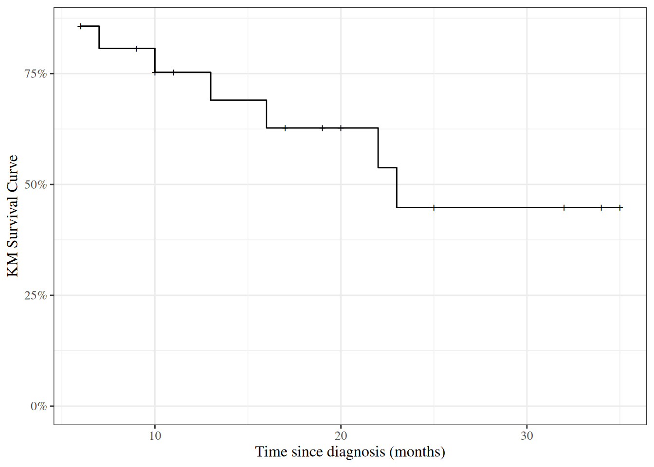
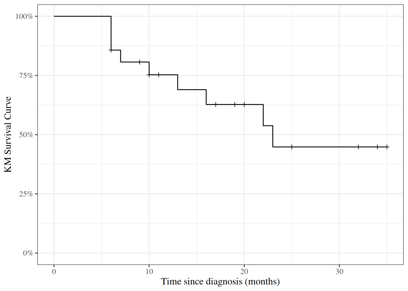
4.8 Likelihood with censoring

If an event time $T$ is observed exactly as $T=t$, then the likelihood of that observation is just its probability density function:

\[ \begin{aligned} \mathscr{L}(t) &= \operatorname{f}(T=t)\\ &\stackrel{\text{def}}{=}\operatorname{f}_T(t)\\ &= {\lambda}_T(t)\operatorname{S}_T(t)\\ \ell(t) &\stackrel{\text{def}}{=}\operatorname{log}\mathopen{}\left\{\mathscr{L}(t)\right\}\mathclose{}\\ &= \operatorname{log}\mathopen{}\left\{{\lambda}_T(t) \operatorname{S}_T(t)\right\}\mathclose{}\\ &= \operatorname{log}\mathopen{}\left\{{\lambda}_T(t)\right\}\mathclose{} + \operatorname{log}\mathopen{}\left\{\operatorname{S}_T(t)\right\}\mathclose{}\\ &= \operatorname{log}\mathopen{}\left\{{\lambda}_T(t)\right\}\mathclose{} - {\Lambda}_T(t)\\ \end{aligned} \]

If instead the event time $T$ is censored and only known to be after time $y$, then the likelihood of that censored observation is instead the survival function evaluated at the censoring time:

\[ \begin{aligned} \mathscr{L}(y) &=p_T(T>y)\\ &\stackrel{\text{def}}{=}\operatorname{S}_T(y)\\ \ell(y) &\stackrel{\text{def}}{=}\operatorname{log}\mathopen{}\left\{\mathscr{L}(y)\right\}\mathclose{}\\ &=\operatorname{log}\mathopen{}\left\{\operatorname{S}(y)\right\}\mathclose{}\\ &=-{\Lambda}(y)\\ \end{aligned} \]

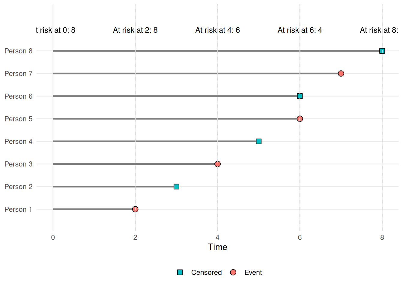
What’s written above is incomplete. We also observed whether or not the observation was censored. Let $C$ denote the time when censoring would occur (if the event did not occur first); let $f_C(y)$ and $S_C(y)$ be the corresponding density and survival functions for the censoring event.

Let $Y$ denote the time when observation ended (either by censoring or by the event of interest occurring), and let $D$ be an indicator variable for the event occurring at $Y$ (so $D=0$ represents a censored observation and $D=1$ represents an uncensored observation). In other words, let $Y \stackrel{\text{def}}{=}\min(T,C)$ and $D \stackrel{\text{def}}{=}\mathbb 1{\{T<=C\}}$.

Then the complete likelihood of the observed data $(Y,D)$ is:

\[ \begin{aligned} \mathscr{L}(y,d) &= \operatorname{p}(Y=y, D=d)\\ &= \mathopen{}\left[\operatorname{p}(T=y,C> y)\right]\mathclose{}^d \cdot \mathopen{}\left[\operatorname{p}(T>y,C=y)\right]\mathclose{}^{1-d}\\ \end{aligned} \]

Typically, survival analyses assume that $C$ and $T$ are mutually independent; this assumption is called “non-informative” censoring.

Then the joint likelihood $\operatorname{p}(Y,D)$ factors into the product $\operatorname{p}(Y), \operatorname{p}(D)$, and the likelihood reduces to:

\[ \begin{aligned} \mathscr{L}(y,d) &= \mathopen{}\left[\operatorname{p}(T=y,C> y)\right]\mathclose{}^d\cdot \mathopen{}\left[\operatorname{p}(T>y,C=y)\right]\mathclose{}^{1-d}\\ &= \mathopen{}\left[\operatorname{p}(T=y)\operatorname{p}(C> y)\right]\mathclose{}^d\cdot \mathopen{}\left[\operatorname{p}(T>y)\operatorname{p}(C=y)\right]\mathclose{}^{1-d}\\ &= \mathopen{}\left[\operatorname{f}_T(y)\operatorname{S}_C(y)\right]\mathclose{}^d\cdot \mathopen{}\left[\operatorname{S}(y)\operatorname{f}_C(y)\right]\mathclose{}^{1-d}\\ &= \mathopen{}\left[\operatorname{f}_T(y)^d \operatorname{S}_C(y)^d\right]\mathclose{}\cdot \mathopen{}\left[\operatorname{S}_T(y)^{1-d} \operatorname{f}_C(y)^{1-d}\right]\mathclose{}\\ &= \mathopen{}\left(\operatorname{f}_T(y)^d \cdot \operatorname{S}_T(y)^{1-d}\right)\mathclose{}\cdot \mathopen{}\left(\operatorname{f}_C(y)^{1-d} \cdot \operatorname{S}_C(y)^{d}\right)\mathclose{} \end{aligned} \]

The corresponding log-likelihood is:

\[ \begin{aligned} \ell(y,d) &= \operatorname{log}\mathopen{}\left\{\mathscr{L}(y,d)\right\}\mathclose{}\\ &= \operatorname{log}\mathopen{}\left\{ \mathopen{}\left(f_T(y)^d \cdot S_T(y)^{1-d}\right)\mathclose{} \cdot \mathopen{}\left(f_C(y)^{1-d} \cdot S_C(y)^{d}\right)\mathclose{} \right\}\mathclose{} \\ &= \operatorname{log}\mathopen{}\left\{f_T(y)^d \cdot S_T(y)^{1-d}\right\}\mathclose{} + \operatorname{log}\mathopen{}\left\{f_C(y)^{1-d} \cdot S_C(y)^{d}\right\}\mathclose{} \end{aligned} \] Let

$\theta_T$ represent the parameters of $p_T(t)$,
$\theta_C$ represent the parameters of $p_C(c)$,
$\theta = (\theta_T, \theta_C)$ be the combined vector of all parameters.

The corresponding score function is:

\[ \begin{aligned} \ell'(y,d) &= \frac{\partial}{\partial \theta} \mathopen{}\left[ \operatorname{log}\mathopen{}\left\{f_T(y)^d \cdot S_T(y)^{1-d}\right\}\mathclose{} + \operatorname{log}\mathopen{}\left\{f_C(y)^{1-d} \cdot S_C(y)^{d}\right\}\mathclose{} \right]\mathclose{} \\ &= \mathopen{}\left( \frac{\partial}{\partial \theta} \operatorname{log}\mathopen{}\left\{ f_T(y)^d \cdot S_T(y)^{1-d} \right\}\mathclose{} \right)\mathclose{} + \mathopen{}\left( \frac{\partial}{\partial \theta} \operatorname{log}\mathopen{}\left\{ f_C(y)^{1-d} \cdot S_C(y)^{d} \right\}\mathclose{} \right)\mathclose{} \end{aligned} \]

As long as $\theta_C$ and $\theta_T$ don’t share any parameters, then if censoring is non-informative, the partial derivative with respect to $\theta_T$ is:

\[ \begin{aligned} \ell'_{\theta_T}(y,d) &\stackrel{\text{def}}{=}\frac{\partial}{\partial \theta_T}\ell(y,d)\\ &= \left( \frac{\partial}{\partial \theta_T} \text{log}\left\{ f_T(y)^d \cdot S_T(y)^{1-d} \right\} \right) + \left( \frac{\partial}{\partial \theta_T} \text{log}\left\{ f_C(y)^{1-d} \cdot S_C(y)^{d} \right\} \right)\\ &= \left( \frac{\partial}{\partial \theta_T} \text{log}\left\{ f_T(y)^d \cdot S_T(y)^{1-d} \right\} \right) + 0\\ &= \frac{\partial}{\partial \theta_T} \text{log}\left\{ f_T(y)^d \cdot S_T(y)^{1-d} \right\}\\ \end{aligned} \]

Thus, the MLE for $\theta_T$ won’t depend on $\theta_C$, and we can ignore the distribution of $C$ when estimating the parameters of $f_T(t)=p(T=t)$.

Then:

\[ \begin{aligned} \mathscr{L}(y,d) &= f_T(y)^d \cdot S_T(y)^{1-d}\\ &= \left(h_T(y)^d S_T(y)^d\right) \cdot S_T(y)^{1-d}\\ &= h_T(y)^d \cdot S_T(y)^d \cdot S_T(y)^{1-d}\\ &= h_T(y)^d \cdot S_T(y)\\ &= S_T(y) \cdot h_T(y)^d \\ \end{aligned} \]

That is, if the event occurred at time $y$ (i.e., if $d=1$), then the likelihood of $(Y,D) = (y,d)$ is equal to the hazard function at $y$ times the survival function at $y$. Otherwise, the likelihood is equal to just the survival function at $y$.

The corresponding log-likelihood is:

\[ \begin{aligned} \ell(y,d) &=\text{log}\left\{\mathscr{L}(y,d)\right\}\\ &= \text{log}\left\{S_T(y) \cdot h_T(y)^d\right\}\\ &= \text{log}\left\{S_T(y)\right\} + \text{log}\left\{h_T(y)^d\right\}\\ &= \text{log}\left\{S_T(y)\right\} + d\cdot \text{log}\left\{h_T(y)\right\}\\ &= -H_T(y) + d\cdot \text{log}\left\{h_T(y)\right\}\\ \end{aligned} \]

In other words, the log-likelihood contribution from a single observation $(Y,D) = (y,d)$ is equal to the negative cumulative hazard at $y$, plus the log of the hazard at $y$ if the event occurred at time $y$.

5 Parametric Models for Time-to-Event Outcomes

5.1 Exponential Distribution

The exponential distribution is the base distribution for survival analysis.
The distribution has a constant hazard ${\lambda}$
The mean survival time is ${\lambda}^{-1}$

Mathematical details of exponential distribution

\[ \begin{aligned} f(t) &= {\lambda}\text{e}^{-{\lambda}t} \\ F(t) &= 1-\text{e}^{-{\lambda}t}\\ \operatorname{S}(t)&= \text{e}^{-{\lambda}t}\\ \operatorname{log}\mathopen{}\left\{\operatorname{S}(t)\right\}\mathclose{}&=-{\lambda}t\\ {\lambda}(t) &= \frac{f(t)}{\operatorname{S}(t)} = \frac{{\lambda}\text{e}^{-{\lambda}t}}{\text{e}^{-{\lambda}t}}={\lambda} \\ E(t) &= {\lambda}^{-1} \\ Var(t) &= {\lambda}^{-2} \\ \operatorname{log}\mathopen{}\left\{f(t)\right\}\mathclose{} &= \operatorname{log}\mathopen{}\left\{{\lambda}\right\}\mathclose{} - {\lambda}t \\ \frac{\partial}{\partial {\lambda}} \operatorname{log}\mathopen{}\left\{f(t)\right\}\mathclose{} &= {\lambda}^{-1} - t \\ &= \operatorname{E}\mathopen{}\left[t\right]\mathclose{} - t \\ &= -(\operatorname{E}\mathopen{}\left[t\right]\mathclose{} - t) \\ &= -\varepsilon \end{aligned} \]

Prediction intervals for time-to-event outcomes

Exercise 3 (Construct a prediction interval) Suppose a cancer patient is predicted to have an expected (mean) lifetime of 7 years after diagnosis, and suppose the distribution is exponential.

Construct a 95% prediction interval for survival.

Tip

Use the quantiles of the exponential distribution.

Solution

Solution 8. If the mean is 7 years until death, then the rate parameter ${\lambda}= 1/7$ events (deaths) per year.

The 0.025 quantile of the exponential distribution with ${\lambda}= 1/7$ is qexp(p 0.025, rate = 1/7) = 0.177225 and the 0.975 quantile is qexp(p 0.975, rate = 1/7) = 25.822156, so the prediction interval is qexp(p c(.025, 0.975), rate = 1/7) = (0.177225, 25.822156).

Exercise 4 Graph the prediction interval as a function of the mean, for Gaussian ($\sigma = 1$), Binomial, Poisson, and Exponential.

Solution

Solution 9. Left to the reader for now.

Exercise 5 (Explain the results) Why do time-to-event models have such wide predictive intervals?

Tip

Consider the relationship between the mean, variance, and standard deviation of the exponential distribution, and contrast that relationship with the Poisson distribution and the Bernoulli distribution.

Solution

Solution 10. In the exponential distribution, variance is the square of the mean (hence SD is equal to mean); as opposed to Poisson, where variance was equal to the mean (and SD is the square-root of the mean), or the Bernoulli, where the variance is the mean minus the square of the mean (so the SD is smaller than the square-root of the mean).

Estimating ${\lambda}$

Suppose we have $m$ exponential survival times of $t_1, t_2,\ldots,t_m$ and $k$ right-censored values at $u_1,u_2,\ldots,u_k$.
A survival time of $t_i=10$ means that subject $i$ died at time 10. A right-censored time $u_i=10$ means that at time 10, subject $i$ was still alive and that we have no further follow-up.
For the moment we will assume that the survival distribution is exponential and that all the subjects have the same parameter ${\lambda}$.

We have $m$ exponential survival times of $t_1, t_2,\ldots,t_m$ and $k$ right-censored values at $u_1,u_2,\ldots,u_k$. The log-likelihood of an observed survival time $t_i$ is \[ \operatorname{log}\mathopen{}\left\{{\lambda}\text{e}^{-{\lambda}t_i}\right\}\mathclose{} = \operatorname{log}\mathopen{}\left\{{\lambda}\right\}\mathclose{}-{\lambda}t_i \] and the likelihood of a censored value is the probability of that outcome (survival greater than $u_j$) so the log-likelihood is

\[ \begin{aligned} \ell_j({\lambda}) &= \operatorname{log}\mathopen{}\left\{\text{e}^{-{\lambda}u_j}\right\}\mathclose{} \\ &= -{\lambda}u_j \end{aligned} \]

Theorem 9 (MLE of the exponential rate parameter) Let $T=\sum t_i$ and $U=\sum u_j$. Then:

\[ \hat{{\lambda}}_{ML} = \frac{m}{T+U} \tag{2}\]

Proof

Proof. \[ \begin{aligned} \ell({\lambda}) &= \sum_{i=1}^m(\operatorname{log}\mathopen{}\left\{{\lambda}\right\}\mathclose{}-{\lambda}t_i) + \sum_{j=1}^k (-{\lambda}u_j)\\ &= m \operatorname{log}\mathopen{}\left\{{\lambda}\right\}\mathclose{} -(T+U){\lambda}\\ \ell'({\lambda}) &=m{\lambda}^{-1} -(T+U)\\ \hat{{\lambda}} &= \frac{m}{T+U} \end{aligned} \]

\[ \begin{aligned} \ell''&=-m/{\lambda}^2\\ &< 0\\ \hat E[T] &= \hat{\lambda}^{-1}\\ &= \frac{T+U}{m} \end{aligned} \]

Fisher Information and Standard Error

\[ \begin{aligned} \operatorname{E}\mathopen{}\left[-\ell''\right]\mathclose{} & = m/{\lambda}^2\\ \operatorname{Var}\mathopen{}\left(\hat{\lambda}\right)\mathclose{} &\approx \mathopen{}\left(\operatorname{E}\mathopen{}\left[-\ell''\right]\mathclose{}\right)^{-1}\mathclose{}\\ &={\lambda}^2/m\\ \text{SE}\left(\hat{\lambda}\right) &= \sqrt{\operatorname{Var}\mathopen{}\left(\hat{\lambda}\right)\mathclose{}}\\ &\approx {\lambda}/\sqrt{m} \end{aligned} \]

$\hat{\lambda}$ depends on the censoring times of the censored observations, but $\operatorname{Var}\mathopen{}\left(\hat{\lambda}\right)\mathclose{}$ only depends on the number of uncensored observations, $m$, and not on the number of censored observations ($k$).

5.2 Other Parametric Survival Distributions

Any density on $[0,\infty)$ can be a survival distribution, but the most useful ones are all skew right.
The most frequently used generalization of the exponential is the Weibull.
Other common choices are the gamma, log-normal, log-logistic, Gompertz, inverse Gaussian, and Pareto.
Most of what we do going forward is non-parametric or semi-parametric, but sometimes these parametric distributions provide a useful approach.

6 Nonparametric Survival Analysis

6.1 Basic ideas

Mostly, we work without a parametric model.
The first task is to estimate a survival function from data listing survival times, and censoring times for censored data.
For example one patient may have relapsed at 10 months. Another might have been followed for 32 months without a relapse having occurred (censored).
The minimum information we need for each patient is a time and a censoring variable which is 1 if the event occurred at the indicated time and 0 if this is a censoring time.

Exm

Example 8 (Clinical Trial for Pediatric Acute Leukemia)

Overview of study

This is from a clinical trial in 1963 for 6-MP treatment vs. placebo for acute leukemia in 42 children (Freireich et al. 1963).

Pairs of children:
matched by remission status at the time of treatment (remstat: 1 = partial, 2 = complete)
randomized to 6-MP (exit times in t2) or placebo (exit times in t1)
Followed until relapse or end of study.
All of the placebo group relapsed, but some of the 6-MP group were censored (which means they were still in remission); indicated by relapse variable (0 = censored, 1 = relapse).
6-MP = 6-Mercaptopurine (Purinethol) is an anti-cancer (“antineoplastic” or “cytotoxic”) chemotherapy drug used currently for Acute lymphoblastic leukemia (ALL). It is classified as an antimetabolite.

Study design

Clinical trial in 1963 for 6-MP treatment vs. placebo for Acute Leukemia in 42 children.
Pairs of children:
matched by remission status at the time of treatment (remstat)
remstat = 1: partial
remstat = 2: complete
randomized to 6-MP (exit time: t2) or placebo (t1).
Followed until relapse or end of study.
All of the placebo group relapsed,
Some of the 6-MP group were censored.

Show R code

library(KMsurv)
data(drug6mp)
drug6mp <- drug6mp |> tibble::as_tibble()
drug6mp

Table 1: drug6mp pediatric acute leukemia data

Data documentation for `drug6mp`

Show R code

# library(printr) # inserts help-file output into markdown output
library(KMsurv)
?drug6mp

Descriptive Statistics

Table 2: Summary statistics for drug6mp data

Show R code

summary(drug6mp)
#>       pair       remstat           t1              t2          relapse     
#>  Min.   : 1   Min.   :1.00   Min.   : 1.00   Min.   : 6.0   Min.   :0.000  
#>  1st Qu.: 6   1st Qu.:2.00   1st Qu.: 4.00   1st Qu.: 9.0   1st Qu.:0.000  
#>  Median :11   Median :2.00   Median : 8.00   Median :16.0   Median :0.000  
#>  Mean   :11   Mean   :1.76   Mean   : 8.67   Mean   :17.1   Mean   :0.429  
#>  3rd Qu.:16   3rd Qu.:2.00   3rd Qu.:12.00   3rd Qu.:23.0   3rd Qu.:1.000  
#>  Max.   :21   Max.   :2.00   Max.   :23.00   Max.   :35.0   Max.   :1.000

The average time in each group is not useful. Some of the 6-MP patients have not relapsed at the time recorded, while all of the placebo patients have relapsed.
The median time is not really useful either because so many of the 6-MP patients have not relapsed (12/21).
Both are biased down in the 6-MP group. Remember that lower times are worse since they indicate sooner recurrence.

Exponential model

We can compute the hazard rate, assuming an exponential model: number of relapses divided by the sum of the exit times (Equation 2).

\[\hat{\lambda}= \frac{\sum_{i=1}^nD_i}{\sum_{i=1}^nY_i}\]

For the placebo, that is just the reciprocal of the mean time:

\[ \begin{aligned} \hat {\lambda}_{\text{placebo}} &= \frac{\sum_{i=1}^nD_i}{\sum_{i=1}^nY_i} \\ &= \frac{\sum_{i=1}^n1}{\sum_{i=1}^nY_i} \\ &= \frac{n}{\sum_{i=1}^nY_i} \\ &= \frac{1}{\bar{Y}} \\ &= \frac{1}{8.666667} \\ &= 0.115385 \end{aligned} \]

For the 6-MP group, $\hat{\lambda}= 9/359 = 0.025$

\[ \begin{aligned} \hat {\lambda}_{\text{6-MP}} &= \frac{\sum_{i=1}^nD_i}{\sum_{i=1}^nY_i} \\ &= \frac{9}{359} \\ &= 0.02507 \end{aligned} \]

The estimated hazard in the placebo group is 4.6 times as large as in the 6-MP group (assuming the hazard is constant over time).

7 The Kaplan-Meier Product Limit Estimator

7.1 Estimating survival in datasets without censoring

In the drug6mp dataset, the estimated survival function for the placebo patients is easy to compute. For any time $t$ in months, $\operatorname{S}(t)$ is the fraction of patients with times greater than $t$:

7.2 Estimating survival in datasets with censoring

For the 6-MP patients, we cannot ignore the censored data because we know that the time to relapse is greater than the censoring time.
For any time $t$ in months, we know that 6-MP patients with times greater than $t$ have not relapsed, and those with relapse time less than $t$ have relapsed, but we don’t know if patients with censored time less than $t$ have relapsed or not.
The procedure we usually use is the Kaplan-Meier product-limit estimator of the survival function.
The Kaplan-Meier estimator is a step function (like the empirical cdf), which changes value only at the event times, not at the censoring times.
At each event time $t_i$, we compute the at-risk set, which includes all observations whose event time or censoring time is at least $t_i$. Its size is $r_i$.
If $d_i$ of the observations have an event time (not a censoring time) of $t_i$, then the group of survivors immediately following time $t_i$ is reduced by the fraction \[\frac{r_i-d_i}{r_i}=1-\frac{d_i}{r_i}\]

Show R code

risk_cartoon <- tibble::tibble(
  person = paste("Person", 1:8),
  exit_time = c(2, 3, 4, 5, 6, 6, 7, 8),
  status = c(
    "Event",
    "Censored",
    "Event",
    "Censored",
    "Event",
    "Censored",
    "Event",
    "Censored"
  )
) |>
  dplyr::mutate(person_id = dplyr::row_number())

risk_counts <- tibble::tibble(time = c(0, 2, 4, 6, 8)) |>
  dplyr::mutate(
    at_risk = purrr::map_int(
      time,
      \(current_time) sum(risk_cartoon$exit_time >= current_time)
    ),
    label = paste0("At risk at ", time, ": ", at_risk)
  )

ggplot2::ggplot(risk_cartoon) +
  ggplot2::aes(y = person_id) +
  ggplot2::geom_segment(
    ggplot2::aes(
      x = 0,
      xend = exit_time,
      yend = person_id
    ),
    linewidth = 1,
    color = "grey50"
  ) +
  ggplot2::geom_point(
    ggplot2::aes(
      x = exit_time,
      shape = status,
      fill = status
    ),
    size = 3,
    color = "black"
  ) +
  ggplot2::geom_vline(
    data = dplyr::filter(risk_counts, time > 0),
    ggplot2::aes(xintercept = time),
    linetype = "dashed",
    color = "grey85"
  ) +
  ggplot2::geom_text(
    data = risk_counts,
    ggplot2::aes(
      x = time,
      y = max(risk_cartoon$person_id) + 0.8,
      label = label
    ),
    size = 3.4,
    vjust = 0
  ) +
  ggplot2::scale_shape_manual(values = c(Event = 21, Censored = 22)) +
  ggplot2::scale_fill_manual(
    values = c(Event = "#F8766D", Censored = "#00BFC4")
  ) +
  ggplot2::scale_y_continuous(
    breaks = risk_cartoon$person_id,
    labels = risk_cartoon$person
  ) +
  ggplot2::coord_cartesian(ylim = c(0.5, max(risk_cartoon$person_id) + 1.6)) +
  ggplot2::labs(
    x = "Time",
    y = NULL,
    shape = NULL,
    fill = NULL
  ) +
  ggplot2::theme_minimal() +
  ggplot2::theme(
    legend.position = "bottom",
    panel.grid.minor = ggplot2::element_blank()
  )

Figure 10: Cartoon risk-set view showing individual follow-up lines. Filled circles indicate events, filled squares indicate censoring times, and dashed lines mark selected times. Labels above show the number at risk at each marked time.

Definition 11 (Risk Set) For a survival study with $n$ subjects, let $T_i$ denote the true event time and $C_i$ the censoring time for subject $i$, and let $\tilde{T}_i = \min(T_i, C_i)$ be the observed follow-up time. The risk set at time $t$ is

\[\mathcal{R}(t) \;\stackrel{\text{def}}{=}\; \bigl\{i \in \{1, \ldots, n\} : \tilde{T}_i \geq t\bigr\},\]

the set of subjects still under observation (neither having experienced the event nor been censored) immediately before time $t$.

The number at risk at time $t$ is

\[r(t) \;\stackrel{\text{def}}{=}\; \lvert \mathcal{R}(t) \rvert.\]

At each ordered event time $t_i$, this count is written $r_i \stackrel{\text{def}}{=}r(t_i)$.

Exm

Example 9 In Figure 10, the 8-person study has $\tilde{T}_i \in \{2, 3, 4, 5, 6, 6, 7, 8\}$. At time $t = 4$, subjects 3, 4, 5, 6, 7, and 8 still have $\tilde{T}_i \geq 4$, so $\mathcal{R}(4) = \{3, 4, 5, 6, 7, 8\}$ and $r(4) = 6$.

Definition 12 (Kaplan-Meier Product-Limit Estimator of Survival Function) If a time-to-event data set contains $k$ event times $t_i$, ($i \in {1:k}$), where $r_i$ is the number of individuals at risk at time $t_i$ and $d_i$ is the number of events at time $t_i$, then the Kaplan-Meier Product-Limit Estimator of the survival function is:

\[\hat{{\lambda}}_i = \frac{d_i}{r_i}\]

\[\hat{\kappa}_i = 1 - \hat{{\lambda}}_i = \frac{r_i - d_i}{r_i}\]

\[\mathop{\hat{\operatorname{S}}}\nolimits_{KM}(t) \stackrel{\text{def}}{=}\prod_{\mathopen{}\left\{i:\ t_i \le t\right\}\mathclose{}} \hat{\kappa}_i\]

To see why multiplying the conditional survival factors estimates marginal survival, write the ordered distinct exit times as $y_1 < y_2 < \cdots < y_m$. Here $Y$ denotes exit time (either event time or censoring time), while $T$ denotes the underlying event time, which is not always observed.

Because $y_{j-1}$ and $y_j$ are consecutive distinct exit times, there are no exits between them. Therefore the conditional probability of surviving between these two times is 1:

\[ \Pr(Y \geq y_j \mid Y > y_{j-1}) = 1. \]

Then the event $\{Y \geq y_j\}$ is contained in the event $\{Y > y_{j-1}\}$, because $y_j > y_{j-1}$. Therefore intersecting $\{Y \geq y_j\}$ with $\{Y > y_{j-1}\}$ does not change the event:

Theorem 10 (Consecutive Exit-Time Identity) If $\Pr(Y \geq y_j \mid Y > y_{j-1}) = 1$, then:

\[\Pr(Y \geq y_j) = \Pr(Y > y_{j-1})\]

Proof

Proof. \[ \begin{aligned} \Pr(Y \geq y_j) \\ &= \Pr(Y \geq y_j, Y > y_{j-1}) \\ &= \Pr(Y \geq y_j \mid Y > y_{j-1}) \Pr(Y > y_{j-1}) \\ &= 1 \Pr(Y > y_{j-1}) \\ &= \Pr(Y > y_{j-1}) \end{aligned} \]

The first equality uses the containment $\{Y \geq y_j\} \subseteq \{Y > y_{j-1}\}$ (subset property). The second equality uses the multiplication rule for probabilities, and the third equality uses the between-exit-time survival assumption.

Let $\kappa(y_j) = \Pr(Y > y_j \mid Y \geq y_j)$ denote the conditional probability of surviving past the exit time $y_j$, given survival up to $y_j$. The marginal survival through $y_j$ can then be written recursively:

\[ \begin{aligned} \operatorname{S}\mathopen{}\left(y_j\right)\mathclose{} &=\Pr(Y > y_j) \\ &= \Pr(Y > y_j, Y \geq y_j)\\ &= \Pr(Y > y_j \mid Y \geq y_j)\Pr(Y \geq y_j)\\ &= \Pr(Y > y_j \mid Y \geq y_j)\Pr(Y > y_{j-1})\\ &= \kappa(y_j)\Pr(Y > y_{j-1}) \\ &= \kappa(y_j)\operatorname{S}\mathopen{}\left(y_{j-1}\right)\mathclose{}. \end{aligned} \]

Here the first equality again uses the subset property: if $Y > y_j$, then $Y \geq y_j$, so $\{Y > y_j\} \subseteq \{Y \geq y_j\}$. The third equality substitutes the Theorem 10 result, $\Pr(Y \geq y_j) = \Pr(Y > y_{j-1})$.

The same recursion can be applied repeatedly. If $S_j = \Pr(Y > y_j)$ and $S_0 = 1$, then:

\[ \begin{aligned} S_1 &= \kappa(y_1)S_0\\ &= \kappa(y_1),\\ S_2 &= \kappa(y_2)S_1\\ &= \kappa(y_2)\kappa(y_1),\\ S_3 &= \kappa(y_3)S_2\\ &= \kappa(y_3)\kappa(y_2)\kappa(y_1). \end{aligned} \]

Continuing in this way gives $S_j = \prod_{k=1}^j \kappa(y_k)$.

To estimate the survival function for the underlying event time $T$, we replace the conditional survival probabilities $\Pr(T > y_k \mid T \geq y_k)$ with their empirical estimates at the observed exit times. This gives the Kaplan-Meier product-limit estimator:

\[ \begin{aligned} \hat{\Pr}(T > t) &= \hat{S}_{KM}(t)\\ &= \prod_{k:\, y_k \leq t} \hat{\Pr}(T > y_k \mid T \geq y_k)\\ &= \prod_{k:\, y_k \leq t} \hat{\kappa}_k\\ &= \prod_{k:\, y_k \leq t} \frac{r_k - d_k}{r_k} \end{aligned} \]

where $r_k$ is the number at risk at time $y_k$ and $d_k$ is the number of events (not total exits) at time $y_k$. The empirical factor $(r_k - d_k)/r_k$ estimates $\Pr(T > y_k \mid T \geq y_k)$ by counting only events in the numerator, since censoring times do not provide information about the event time distribution.

For any time $t$ between two consecutive exit times, the estimate stays constant, because the only additional conditional survival factors are 1.

Exercise 6 Table 3 lists some simulated survival data, where:

$Y$ is study exit time
$D$ is reason for study exit:
- $D=1$: event
- $D=0$: censored
S is the combination of $Y$ and $D$ into a single Surv() variable.

Show R code

library(tibble)
data1 <- tibble(
  Y = c(1, 3, 7, 10, 13, 15, 16, 16, 16),
  D = c(1, 1, 1,  1,  0,  1,  0,  0,  0),
  S = survival::Surv(Y, D)
)
knitr::kable(data1)

Table 3: Simulated survival data for Exercise 6.

Y	D	S
1	1	1
3	1	3
7	1	7
10	1	10
13	0	13+
15	1	15
16	0	16+
16	0	16+
16	0	16+

Compute the Kaplan-Meier (KM) estimated survival curve by hand.

Solution

Solution 4. Let:

$n$: total sample size
$y$: study exit time;
$d(y)$: number of events at $y$;
$c(y)$: number exiting without events (“censored”) at $y$;
$e(y) = d(y) + c(y)$: total exiting at $y$;
$E(y)$: cumulative exits prior to $y$;
$r(y) = n - E(y)$: number at risk at $y$;
$r^*(y) = r(y) - e(y)$: number at risk after $y$;
$\hat{\kappa}(y) = \hat{\Pr}(T > y \mid T \geq y) = [r(y) - d(y)]/r(y)$: conditional survival factor;
$\hat{{\lambda}}(y) = \hat{\Pr}(T = y \mid T \geq y) = \frac{d(y)}{r(y)} = 1 - \hat{\kappa}(y)$: estimated discrete hazard;
$\mathop{\hat{\operatorname{S}}}\nolimits_{KM}(y) = \prod_{k:\, y_k \leq y} \hat{\kappa}(y_k)$: Kaplan-Meier survival estimate.

Show R code

library(pander)
library(tidyverse)

km_curve <-
  data1 |>
  summarise(.by  = Y,
            events = sum(D == 1),
            censored = sum(D == 0)) |>
  arrange(Y) |>
  mutate(
    study_size = nrow(data1),
    exiting = events + censored,
    exited = cumsum(exiting) |> dplyr::lag(default = 0),
    at_risk = study_size - exited,
    r_star = at_risk - exiting,
    hazard = events / at_risk,
    km_factor = 1 - hazard,
    km_surv_curve = cumprod(km_factor)
  ) |>
  select(-study_size) |>
  relocate(km_factor, .before = hazard)
km_curve |>
  mutate(
    hazard_math = paste0("\\frac{", events, "}{", at_risk, "}"),
    km_factor_math = paste0("\\frac{", at_risk - events, "}{", at_risk, "}"),
    km_surv_curve = paste0(
      "$",
      purrr::map_chr(
        row_number(),
        \(i) paste(km_factor_math[seq_len(i)], collapse = " \\times ")
      ),
      " = ",
      round(km_surv_curve, 4),
      "$"
    ),
    hazard = paste0(
      "$", hazard_math, " = ",
      round(hazard, 4), "$"
    ),
    km_factor = paste0(
      "$", km_factor_math, " = ",
      round(km_factor, 4), "$"
    )
  ) |>
  select(-hazard_math, -km_factor_math) |>
  rename(
    `$y$`                        = Y,
    `$d(y)$`                     = events,
    `$c(y)$`                     = censored,
    `$e(y)$`                     = exiting,
    `$E(y)$`                     = exited,
    `$r(y)$`                     = at_risk,
    `$r^*(y)$`                   = r_star,
    `$\\hat{\\cs}(y)$`         = km_factor,
    `$\\hat{\\haz}(y)$`          = hazard,
    `$\\hsurv_{KM}(y)$`          = km_surv_curve
  ) |>
  pander()

Table 4: Kaplan-Meier survival curve calculations

$y$	$d(y)$	$c(y)$	$e(y)$	$E(y)$	$r(y)$	$r^*(y)$	$\hat{\kappa}(y)$	$\hat{{\lambda}}(y)$	$\mathop{\hat{\operatorname{S}}}\nolimits_{KM}(y)$
1	1	0	1	0	9	8	$\frac{8}{9} = 0.8889$	$\frac{1}{9} = 0.1111$	$\frac{8}{9} = 0.8889$
3	1	0	1	1	8	7	$\frac{7}{8} = 0.875$	$\frac{1}{8} = 0.125$	$\frac{8}{9} \times \frac{7}{8} = 0.7778$
7	1	0	1	2	7	6	$\frac{6}{7} = 0.8571$	$\frac{1}{7} = 0.1429$	$\frac{8}{9} \times \frac{7}{8} \times \frac{6}{7} = 0.6667$
10	1	0	1	3	6	5	$\frac{5}{6} = 0.8333$	$\frac{1}{6} = 0.1667$	$\frac{8}{9} \times \frac{7}{8} \times \frac{6}{7} \times \frac{5}{6} = 0.5556$
13	0	1	1	4	5	4	$\frac{5}{5} = 1$	$\frac{0}{5} = 0$	$\frac{8}{9} \times \frac{7}{8} \times \frac{6}{7} \times \frac{5}{6} \times \frac{5}{5} = 0.5556$
15	1	0	1	5	4	3	$\frac{3}{4} = 0.75$	$\frac{1}{4} = 0.25$	$\frac{8}{9} \times \frac{7}{8} \times \frac{6}{7} \times \frac{5}{6} \times \frac{5}{5} \times \frac{3}{4} = 0.4167$
16	0	3	3	6	3	0	$\frac{3}{3} = 1$	$\frac{0}{3} = 0$	$\frac{8}{9} \times \frac{7}{8} \times \frac{6}{7} \times \frac{5}{6} \times \frac{5}{5} \times \frac{3}{4} \times \frac{3}{3} = 0.4167$

Exercise 7 Implement the KM survival curve estimator in R. Check the output of your implementation against the version in the survival package.

Solution

Solution 5. See above for implementation. Here’s the version from the survival package:

Show R code

library(survival)
data1 |>
  survfit(Surv(time = Y, event = D) ~ 1, data = _) |>
  summary()
#> Call: survfit(formula = Surv(time = Y, event = D) ~ 1, data = data1)
#> 
#>  time n.risk n.event survival std.err lower 95% CI upper 95% CI
#>     1      9       1    0.889   0.105        0.706        1.000
#>     3      8       1    0.778   0.139        0.549        1.000
#>     7      7       1    0.667   0.157        0.420        1.000
#>    10      6       1    0.556   0.166        0.310        0.997
#>    15      4       1    0.417   0.173        0.185        0.940

Exercise 8 Graph the KM estimated survival curve for the data in Table 3.

Solution

Solution 6.

Show R code

library(ggplot2)
km_curve |>
  ggplot(aes(x = Y, y = km_surv_curve)) +
  geom_step() +
  geom_point(data = km_curve |> filter(censored > 0), shape = 3) +
  ylab("KM Survival Curve") +
  expand_limits(y = c(0, 1), x = 0) +
  scale_y_continuous(labels = scales::percent)

Show R code

library(ggfortify)
data1 <- data1 |>
  mutate(
    surv = Surv(time = Y, event = D)
  )
KM_model <- data1 |> survfit(formula = surv ~ 1)
KM_model |> autoplot()

Exercise 9 Find the KM estimate of median survival time.

Solution

Solution 7.

Show R code

KM_model |> quantile(prob = 0.5) |> as_tibble()

Theorem 11 (Kaplan-Meier Estimate with No Censored Observations) If there are no censored data, and there are $n$ data points, then just after (say) the third event time

\[ \begin{aligned} \mathop{\hat{\operatorname{S}}}\nolimits(t) &= \prod_{t_i \le t}\mathopen{}\left[1-\frac{d_i}{r_i}\right]\mathclose{} \\ &= \mathopen{}\left[\frac{n-d_1}{n}\right]\mathclose{} \mathopen{}\left[\frac{n-d_1-d_2}{n-d_1}\right]\mathclose{} \mathopen{}\left[\frac{n-d_1-d_2-d_3}{n-d_1-d_2}\right]\mathclose{} \\ &= \frac{n-d_1-d_2-d_3}{n} \\ &=1-\frac{d_1+d_2+d_3}{n} \\ &=1-\hat F(t) \end{aligned} \]

where $\hat F(t)$ is the usual empirical CDF estimate.

7.3 Variance of the Kaplan-Meier estimator

The estimated variance of $\mathop{\hat{\operatorname{S}}}\nolimits(t)$ at a single time point $t$ is given by Greenwood’s formula:

Theorem 12 (Greenwood’s estimator for variance of Kaplan-Meier survival estimator) \[ \mathop{\widehat{\operatorname{Var}}}\nolimits\mathopen{}\left(\mathop{\hat{\operatorname{S}}}\nolimits(t)\right)\mathclose{} = \mathop{\hat{\operatorname{S}}}\nolimits(t)^2\sum_{t_i \le t}\frac{d_i}{r_i(r_i-d_i)} \tag{3}\]

(Klein and Moeschberger 2003, sec. 4.2, eq. (4.2.2))

We can use Equation 3 for confidence intervals for a survival function or a difference of survival functions.

7.3.1 Understanding Greenwood’s formula (optional)

To see where Greenwood’s formula comes from, let $x_i = r_i - d_i$. We approximate the solution treating each time as independent, with $r_i$ fixed and ignore randomness in times of failure and we treat $x_i$ as independent binomials $\text{Bin}(r_i,p_i)$. Letting $\operatorname{S}(t)$ be the “true” survival function

\[ \begin{aligned} \mathop{\hat{\operatorname{S}}}\nolimits(t) &=\prod_{t_i \le t}x_i/r_i\\ \operatorname{S}(t)&=\prod_{t_i \le t}p_i \end{aligned} \]

\[ \begin{aligned} \frac{\mathop{\hat{\operatorname{S}}}\nolimits(t)}{\operatorname{S}(t)} &= \prod_{t_i \le t} \frac{x_i}{p_i r_i} \\ &= \prod_{t_i \le t} \frac{\hat p_i}{p_i} \\ &= \prod_{t_i \le t} \mathopen{}\left(1+\frac{\hat p_i-p_i}{p_i}\right)\mathclose{} \\ &\approx 1+\sum_{t_i \le t} \frac{\hat p_i-p_i}{p_i} \end{aligned} \]

\[ \begin{aligned} \operatorname{Var}\mathopen{}\left(\frac{\mathop{\hat{\operatorname{S}}}\nolimits(t)}{\operatorname{S}(t)}\right)\mathclose{} &\approx \operatorname{Var}\mathopen{}\left(1+\sum_{t_i \le t} \frac{\hat p_i-p_i}{p_i}\right)\mathclose{} \\ &=\sum_{t_i \le t} \frac{1}{p_i^2}\frac{p_i(1-p_i)}{r_i} \\ &= \sum_{t_i \le t} \frac{(1-p_i)}{p_i r_i} \\ &\approx\sum_{t_i \le t} \frac{(1-x_i/r_i)}{x_i} \\ &=\sum_{t_i \le t} \frac{r_i-x_i}{x_i r_i} \\ &=\sum_{t_i \le t} \frac{d_i}{r_i(r_i-d_i)} \\ \therefore\operatorname{Var}\mathopen{}\left(\mathop{\hat{\operatorname{S}}}\nolimits(t)\right)\mathclose{} &\approx \mathop{\hat{\operatorname{S}}}\nolimits(t)^2\sum_{t_i \le t} \frac{d_i}{r_i(r_i-d_i)} \end{aligned} \]

Exm

Example 10 (Kaplan-Meier curve for drug6mp data) Here is the Kaplan-Meier estimated survival curve for the patients who received 6-MP in the drug6mp dataset (we will see code to produce figures like this one shortly):

Show R code

library(KMsurv)
data(drug6mp)
library(dplyr)
library(survival)

km_model1 <-
  drug6mp |>
  mutate(surv = Surv(t2, relapse)) |>
  survfit(formula = surv ~ 1, data = _)

library(ggfortify)
km_model1 |>
  autoplot(
    mark.time = TRUE,
    conf.int = FALSE
  ) +
  expand_limits(y = 0) +
  xlab("Time since diagnosis (months)") +
  ylab("KM Survival Curve")

Figure 11: Kaplan-Meier Survival Curve for 6-MP Patients

7.4 Kaplan-Meier calculations

Let’s compute these estimates and build the chart by hand:

Show R code

library(KMsurv)
library(dplyr)
data(drug6mp)

data_v2 <-
  drug6mp |>
  as_tibble() |>
  mutate(
    remstat = remstat |>
      case_match(
        1 ~ "partial",
        2 ~ "complete"
      ),
    # renaming to "outcome" while relabeling is just a style choice:
    outcome = relapse |>
      case_match(
        0 ~ "censored",
        1 ~ "relapsed"
      )
  )

km_table <-
  data_v2 |>
  summarize(
    .by = t2,
    Relapses = sum(outcome == "relapsed"),
    Censored = sum(outcome == "censored")
  ) |>
  # here we add a start time row, so the graph starts at time 0:
  bind_rows(
    tibble(
      t2 = 0,
      Relapses = 0,
      Censored = 0
    )
  ) |>
  # sort in time order:
  arrange(t2) |>
  mutate(
    Exiting = Relapses + Censored,
    `Study Size` = sum(Exiting),
    Exited = cumsum(Exiting) |> dplyr::lag(default = 0),
    `At Risk` = `Study Size` - Exited,
    Hazard = Relapses / `At Risk`,
    `KM Factor` = 1 - Hazard,
    `Cumulative Hazard` = cumsum(`Hazard`),
    `KM Survival Curve` = cumprod(`KM Factor`)
  )

library(pander)
pander(km_table)

t2	Relapses	Censored	Exiting	Study Size	Exited	At Risk	Hazard	KM Factor	Cumulative Hazard	KM Survival Curve
0	0	0	0	21	0	21	0	1	0	1
6	3	1	4	21	0	21	0.1429	0.8571	0.1429	0.8571
7	1	0	1	21	4	17	0.05882	0.9412	0.2017	0.8067
9	0	1	1	21	5	16	0	1	0.2017	0.8067
10	1	1	2	21	6	15	0.06667	0.9333	0.2683	0.7529
11	0	1	1	21	8	13	0	1	0.2683	0.7529
13	1	0	1	21	9	12	0.08333	0.9167	0.3517	0.6902
16	1	0	1	21	10	11	0.09091	0.9091	0.4426	0.6275
17	0	1	1	21	11	10	0	1	0.4426	0.6275
19	0	1	1	21	12	9	0	1	0.4426	0.6275
20	0	1	1	21	13	8	0	1	0.4426	0.6275
22	1	0	1	21	14	7	0.1429	0.8571	0.5854	0.5378
23	1	0	1	21	15	6	0.1667	0.8333	0.7521	0.4482
25	0	1	1	21	16	5	0	1	0.7521	0.4482
32	0	2	2	21	17	4	0	1	0.7521	0.4482
34	0	1	1	21	19	2	0	1	0.7521	0.4482
35	0	1	1	21	20	1	0	1	0.7521	0.4482

7.4.1 Summary

For the 6-MP patients at time 6 months, there are 21 patients at risk. At $t=6$ there are 3 relapses and 1 censored observations.

The Kaplan-Meier factor is $(21-3)/21 = 0.857$. The number at risk for the next time ($t=7$) is $21-3-1=17$.

At time 7 months, there are 17 patients at risk. At $t=7$ there is 1 relapse and 0 censored observations. The Kaplan-Meier factor is $(17-1)/17 = 0.941$. The Kaplan Meier estimate is $0.857\times0.941=0.807$. The number at risk for the next time ($t=9$) is $17-1=16$.

Now, let’s graph this estimated survival curve using ggplot():

Show R code

library(ggplot2)
conflicts_prefer(dplyr::filter)
km_table |>
  ggplot(aes(x = t2, y = `KM Survival Curve`)) +
  geom_step() +
  geom_point(data = km_table |> filter(Censored > 0), shape = 3) +
  expand_limits(y = c(0, 1), x = 0) +
  xlab("Time since diagnosis (months)") +
  ylab("KM Survival Curve") +
  scale_y_continuous(labels = scales::percent)

Figure 12: KM curve for 6MP patients, calculated by hand

Exercise 10 (Construct a prediction interval) Suppose a cancer patient is predicted to have an expected (mean) lifetime of 7 years after diagnosis, and suppose the distribution is exponential.

Construct a 95% prediction interval for survival.

Tip

Use the quantiles of the exponential distribution.

Solution

Solution 8. If the mean is 7 years until death, then the rate parameter ${\lambda}= 1/7$ events (deaths) per year.

Exercise 11 Graph the prediction interval as a function of the mean, for Gaussian ($\sigma = 1$), Binomial, Poisson, and Exponential.

Solution

Solution 9. Left to the reader for now.

Exercise 12 (Explain the results) Why do time-to-event models have such wide predictive intervals?

Tip

Solution

8 Using the `survival` package in R

We don’t have to do these calculations by hand every time; the survival package and several others have functions available to automate many of these tasks (full list: https://cran.r-project.org/web/views/Survival.html).

8.1 The `Surv` function

To use the survival package, the first step is telling R how to combine the exit time and exit reason (censoring versus event) columns. The Surv() function accomplishes this task.

Exm

Example 11 (Surv() with drug6mp data)

Show R code

library(survival)
data_v3 <-
  data_v2 |>
  mutate(
    surv2 = Surv(
      time = t2,
      event = (outcome == "relapsed")
    )
  )

print(data_v3)
#> # A tibble: 21 × 7
#>     pair remstat     t1    t2 relapse outcome   surv2
#>    <int> <chr>    <int> <int>   <int> <chr>    <Surv>
#>  1     1 partial      1    10       1 relapsed    10 
#>  2     2 complete    22     7       1 relapsed     7 
#>  3     3 complete     3    32       0 censored    32+
#>  4     4 complete    12    23       1 relapsed    23 
#>  5     5 complete     8    22       1 relapsed    22 
#>  6     6 partial     17     6       1 relapsed     6 
#>  7     7 complete     2    16       1 relapsed    16 
#>  8     8 complete    11    34       0 censored    34+
#>  9     9 complete     8    32       0 censored    32+
#> 10    10 complete    12    25       0 censored    25+
#> # ℹ 11 more rows

The output of Surv() is a vector of objects with class Surv. When we print this vector:

observations where the event was observed are printed as the event time (for example, surv2 = 10 on line 1)
observations where the event was right-censored are printed as the censoring time with a plus sign (+; for example, surv2 = 32+ on line 3).

8.2 The `survfit` function

Once we have constructed our Surv variable, we can calculate the Kaplan-Meier estimate of the survival curve using the survfit() function.

Note

The documentation for ?survfit isn’t too helpful; the survfit.formula documentation is better.

Exm

Example 12 (survfit() with drug6mp data) Here we use survfit() to create a survfit object, which contains the Kaplan-Meier estimate:

Show R code

km_model <- survfit(
  formula = surv2 ~ 1,
  data = data_v3
)

print.survfit() just gives some summary statistics:

Show R code

print(km_model)
#> Call: survfit(formula = surv2 ~ 1, data = data_v3)
#> 
#>       n events median 0.95LCL 0.95UCL
#> [1,] 21      9     23      16      NA

summary.survfit() shows us the underlying Kaplan-Meier table:

Show R code

summary(km_model)
#> Call: survfit(formula = surv2 ~ 1, data = data_v3)
#> 
#>  time n.risk n.event survival std.err lower 95% CI upper 95% CI
#>     6     21       3    0.857  0.0764        0.720        1.000
#>     7     17       1    0.807  0.0869        0.653        0.996
#>    10     15       1    0.753  0.0963        0.586        0.968
#>    13     12       1    0.690  0.1068        0.510        0.935
#>    16     11       1    0.627  0.1141        0.439        0.896
#>    22      7       1    0.538  0.1282        0.337        0.858
#>    23      6       1    0.448  0.1346        0.249        0.807

We can specify which time points we want using the times argument:

Show R code

summary(
  km_model,
  times = c(0, data_v3$t2)
)
#> Call: survfit(formula = surv2 ~ 1, data = data_v3)
#> 
#>  time n.risk n.event survival std.err lower 95% CI upper 95% CI
#>     0     21       0    1.000  0.0000        1.000        1.000
#>    10     15       1    0.753  0.0963        0.586        0.968
#>     7     17       1    0.807  0.0869        0.653        0.996
#>    32      4       0    0.448  0.1346        0.249        0.807
#>    23      6       1    0.448  0.1346        0.249        0.807
#>    22      7       1    0.538  0.1282        0.337        0.858
#>     6     21       3    0.857  0.0764        0.720        1.000
#>    16     11       1    0.627  0.1141        0.439        0.896
#>    34      2       0    0.448  0.1346        0.249        0.807
#>    32      4       0    0.448  0.1346        0.249        0.807
#>    25      5       0    0.448  0.1346        0.249        0.807
#>    11     13       0    0.753  0.0963        0.586        0.968
#>    20      8       0    0.627  0.1141        0.439        0.896
#>    19      9       0    0.627  0.1141        0.439        0.896
#>     6     21       3    0.857  0.0764        0.720        1.000
#>    17     10       0    0.627  0.1141        0.439        0.896
#>    35      1       0    0.448  0.1346        0.249        0.807
#>     6     21       3    0.857  0.0764        0.720        1.000
#>    13     12       1    0.690  0.1068        0.510        0.935
#>     9     16       0    0.807  0.0869        0.653        0.996
#>     6     21       3    0.857  0.0764        0.720        1.000
#>    10     15       1    0.753  0.0963        0.586        0.968

Show R code

?summary.survfit

8.3 Plotting estimated survival functions

We can plot survfit objects with plot(), autoplot(), or ggsurvplot():

Show R code

library(ggfortify)
autoplot(km_model)

Kaplan-Meier Survival Curve for 6-MP Patients

8.3.1 quantiles of survival curve

We can extract quantiles with quantile():

Show R code

km_model |>
  quantile(p = c(.25, .5)) |>
  as_tibble() |>
  mutate(p = c(.25, .5)) |>
  relocate(p, .before = everything())

8.4 R Packages Ecosystem for Survival Analysis

R provides a rich ecosystem of packages for survival analysis, ranging from core functionality to specialized visualization tools and advanced modeling capabilities.

8.4.1 Visualization Packages

ggsurvfit

ggsurvfit is a modern package for creating publication-ready survival plots using ggplot2.

Developed by Daniel D. Sjoberg and collaborators
Seamlessly integrates with ggplot2, allowing full customization using familiar ggplot2 syntax
Key features:
- Create Kaplan-Meier plots with ggsurvfit()
- Add confidence intervals with add_confidence_interval()
- Add risk tables with add_risktable()
- Add quantile annotations with add_quantile()
- Support for competing risks with ggcuminc()
Produces publication-ready legends without showing raw variable names
All plot elements are native ggplot2 layers, making customization straightforward
Available on CRAN and GitHub

survminer

survminer is another popular visualization package for survival analysis.

Creates ggplot2-based survival plots using ggsurvplot()
Provides functions for visualizing Cox model results
Includes tools for testing proportional hazards assumptions
Offers built-in themes and color palettes for publication-quality plots
Can display risk tables, cumulative events, and censoring counts

ggfortify

ggfortify extends ggplot2 with automatic plotting capabilities.

Provides autoplot() method for survfit objects (demonstrated in the plotting example above)
One-line code to create survival curves with confidence intervals
Automatically handles grouping variables and creates legends
Shows censoring marks on plots by default
Returns ggplot2 objects for further customization
Also supports many other statistical objects beyond survival analysis

8.4.2 Additional Modeling Packages

Several packages extend the modeling capabilities beyond the core survival package:

flexsurv: Flexible parametric survival models with a wide range of distributions
rms (Regression Modeling Strategies): Advanced regression modeling including survival models with tools for model validation and calibration
cmprsk: Competing risks regression using the Fine-Gray model
mstate: Multi-state survival models for complex event histories
timereg: Flexible regression models for survival data, including additive hazards models
frailtypack: Frailty models for clustered or recurrent event data
riskRegression: Risk prediction models and performance evaluation
pec: Prediction error curves for survival model validation
prodlim: Fast estimation of survival models including competing risks

8.4.3 Package Selection Guidance

For most standard survival analyses:

Use survival for core functionality (Kaplan-Meier, Cox models, parametric models)
Choose ggsurvfit for modern, customizable survival plots if you’re familiar with ggplot2
Consider survminer as an alternative visualization package with many built-in features
Use ggfortify if you want quick, automatic plots with minimal code

For specialized analyses:

Competing risks: cmprsk or riskRegression
Multi-state models: mstate
Flexible parametric models: flexsurv
Clustered/recurrent events: frailtypack
Model validation: rms or pec

The CRAN Survival Analysis Task View provides the most comprehensive and up-to-date list of available packages.

9 The log-rank test

(a.k.a. the Mantel-Cox test)

Exercise 13 How do we test the null hypothesis that two or more groups have the same time-to-event distribution?

Solution

Solution 11. One option is the log-rank test, which compares the Kaplan-Meier estimates of the survival functions of those groups.

Adapted from (Kleinbaum and Klein 2012, sec. IV, pp. 67–68):

The log-rank test is a large-sample chi-square test.
The log-rank test uses a test statistic that compares KM curves between groups across all survival times.
Like many other statistics used in chi-square tests, the log-rank statistic compares observed versus expected cell counts over categories of outcomes.
The categories for the log-rank statistic are defined by each of the ordered failure times for the entire set of data being analyzed.

9.1 Notation

Suppose we are comparing $G \ge 2$ groups, indexed by $g = 1, \ldots, G$. Pool the failure times across all groups and let

$t_1 < t_2 < \cdots < t_k$ be the distinct ordered failure times in the pooled data ($i = 1, \ldots, k$ indexes these times).

For each ordered failure time $t_i$ and each group $g$, define:

Symbol	Meaning
$d_{gi}$	number of failures in group $g$ at time $t_i$
$r_{gi}$	number at risk in group $g$ just before time $t_i$
$d_i = \sum_{g=1}^{G} d_{gi}$	total failures at $t_i$ (pooled across groups)
$r_i = \sum_{g=1}^{G} r_{gi}$	total at risk at $t_i$ (pooled across groups)

This matches the $(d_i, r_i)$ notation used for the Kaplan-Meier estimator elsewhere in this chapter; here we additionally split each count by group.

Kleinbaum (2012, 67–69) uses $m_{if}$ and $n_{if}$ in place of $d_{gi}$ and $r_{gi}$; we changed letters here to stay consistent with the $(d_i, r_i)$ already used throughout this chapter.

9.2 Expected counts under the null

The null hypothesis is

\[H_0:\; \text{all $G$ groups have the same survival function.}\]

Under $H_0$, the pooled marginal hazard estimate at time $t_i$ is

\[\hat{{\lambda}}_i = \frac{d_i}{r_i}.\]

The expected number of failures in group $g$ at time $t_i$ under $H_0$ is the pooled hazard applied to that group’s risk set (Kleinbaum and Klein 2012, 68, “expected-cell-counts” box):

\[ e_{gi} \;=\; r_{gi}\,\hat{{\lambda}}_i \;=\; \underbrace{\frac{r_{gi}}{r_i}}_{\text{fraction at risk}}\;\cdot\; \underbrace{d_i}_{\text{total failures}} \tag{4}\]

The summed observed minus expected score for group $g$ over all failure times is:

\[O_g - E_g \;\stackrel{\text{def}}{=}\; \sum_{i=1}^{k} \mathopen{}\left(d_{gi} - e_{gi}\right)\mathclose{}.\]

9.3 Log-rank statistic (two groups)

For two groups ($G = 2$), the observed-minus-expected scores satisfy $O_1 - E_1 = -(O_2 - E_2)$ (the total failures at each $t_i$ are by definition partitioned across the two groups), so it does not matter which group we use to form the test statistic.

Theorem 13 (Log-rank statistic, two groups) For either $g \in \{1, 2\}$,

\[ \chi^2_{\text{LR}} \;=\; \frac{(O_g - E_g)^2}{\widehat{\operatorname{Var}\mathopen{}\left(O_g - E_g\right)\mathclose{}}} \;\stackrel{H_0}{\sim}\; \chi^2_1 \tag{5}\]

where $r_{1i}$ and $r_{2i}$ are the at-risk counts for groups 1 and 2 at time $t_i$ (i.e., $r_{gi}$ from Section 9.1 for $g = 1, 2$), and the variance estimate is

\[ \widehat{\operatorname{Var}\mathopen{}\left(O_g - E_g\right)\mathclose{}} \;=\; \sum_{i=1}^{k} \frac{r_{1i}\, r_{2i}\, d_i\, (r_i - d_i)}{r_i^2\,(r_i - 1)}. \tag{6}\]

For two groups, the variance is the same whether computed for group 1 or group 2.

(Kleinbaum and Klein 2012, 69–70, two-group variance formula)

Equation 6 is the hypergeometric variance for the count of failures from group 1 at $t_i$ conditional on $(d_i, r_{1i}, r_{2i})$, summed over failure times. Each summand has the form $r_{1i} r_{2i} d_i (r_i - d_i) / [r_i^2 (r_i - 1)]$.

9.4 Log-rank statistic (more than two groups)

For $G \ge 2$ groups, the log-rank statistic still uses the observed-minus-expected scores $O_g - E_g$, but the variance–covariance matrix of the vector $\mathbf{O} - \mathbf{E} \stackrel{\text{def}}{=}(O_1 - E_1, \ldots, O_G - E_G)'$ is nontrivial because the scores are linearly dependent ($\sum_g (O_g - E_g) = 0$). The statistic takes the matrix-quadratic form

\[ \chi^2_{\text{LR}} \;=\; (\mathbf{O} - \mathbf{E})'\,\widehat{\Sigma}^{-}\,(\mathbf{O} - \mathbf{E}) \;\stackrel{H_0}{\sim}\; \chi^2_{G - 1} \]

where $\widehat\Sigma$ is the estimated variance–covariance matrix of $\mathbf{O} - \mathbf{E}$ and $\widehat\Sigma^{-}$ is a generalized inverse (any $G - 1$ of the rows/columns suffice, since the scores sum to zero).

(Kleinbaum and Klein 2012, 71–72 and Chapter 2 Appendix for the matrix formula)

In practice we don’t compute this by hand — every standard survival package (survival::survdiff in R, sts test in Stata, LIFETEST in SAS) returns the exact log-rank statistic.

9.5 Approximate (Pearson-style) statistic

When only $(O_g, E_g)$ are available — e.g., from a printed summary — the variance–covariance matrix can be replaced by the diagonal $E_g$ entries to yield the classic Pearson-style approximation:

\[X^2 \;\approx\; \sum_{g=1}^{G} \frac{(O_g - E_g)^2}{E_g}.\]

This is what some textbooks call “the log-rank test”; it is approximately equal to the exact statistic.

(Kleinbaum and Klein 2012, 70 (approximate formula))

9.6 The `survdiff` function

Show R code

?survdiff

Exm

Example 13 (survdiff() with drug6mp data) Now we are going to compare the placebo and 6-MP data. We need to reshape the data to make it usable with the standard survival workflow:

Show R code

library(survival)
library(tidyr)
data_v4 <-
  data_v3 |>
  select(pair, remstat, t1, t2, outcome) |>
  # here we are going to change the data from a wide format to long:
  pivot_longer(
    cols = c(t1, t2),
    names_to = "treatment",
    values_to = "exit_time"
  ) |>
  mutate(
    treatment = treatment |>
      case_match(
        "t1" ~ "placebo",
        "t2" ~ "6-MP"
      ),
    outcome = if_else(
      treatment == "placebo",
      "relapsed",
      outcome
    ),
    surv = Surv(
      time = exit_time,
      event = (outcome == "relapsed")
    )
  )

Using this long data format, we can fit a Kaplan-Meier curve for each treatment group simultaneously:

Show R code

km_model2 <-
  survfit(
    formula = surv ~ treatment,
    data = data_v4
  )

We can plot the curves in the same graph:

Show R code

km_model2 |> autoplot()

We can also perform something like a t-test, where the null hypothesis is that the curves are the same. The table below shows the per-time $(d_{gi}, r_{gi})$ counts and the expected counts $e_{gi}$ from Equation 4:

Show R code

o_e <- data_v4 |>
  arrange(exit_time) |>
  mutate(
    .by = treatment,
    n_exited = row_number(),
    n_at_risk = n() - n_exited + 1
  ) |>
  dplyr::summarize(
    .by = all_of(c("exit_time", "treatment")),
    n_at_risk = max(n_at_risk),
    n_events = sum(outcome == "relapsed")
  ) |>
  tidyr::pivot_wider(
    names_from = "treatment",
    values_from = c(n_at_risk, n_events)
  ) |>
  tidyr::fill(
    starts_with("n_at_risk"),
    .direction = "up"
  ) |>
  replace_na(list("n_events_placebo" = 0,
                  "n_events_6-MP" = 0)) |>
  mutate(
    n_at_risk = rowSums(across(starts_with("n_at_risk"))),
    n_events = rowSums(across(starts_with("n_events"))),
    marginal_hazard = n_events / n_at_risk,
    expected_6mp = marginal_hazard * `n_at_risk_6-MP`,
    expected_plc = marginal_hazard * n_at_risk_placebo,
    diff_6mp = `n_events_6-MP` - expected_6mp,
    diff_plc = n_events_placebo - expected_plc
  ) |>
  filter(n_events > 0)

o_e

Table 5: Observed and expected event counts for the 6-MP data, for the log-rank test. Columns: exit_time is $t_i$; n_at_risk_placebo/n_at_risk_6-MP are $r_{gi}$; n_events_placebo/n_events_6-MP are $d_{gi}$; n_at_risk/n_events are pooled $r_i$, $d_i$; marginal_hazard is $\hat{{\lambda}}_i = d_i / r_i$; expected_* are $e_{gi}$ from Equation 4; diff_* are the per-time contributions $d_{gi} - e_{gi}$ to $O_g - E_g$.

The summed observed $O_g$ and expected $E_g$ totals (one row, one column per group):

Show R code

o_e_summ <- o_e |>
  summarize(
    across(starts_with("expected"), sum),
    across(starts_with("n_events_"), sum)
  )
pander::pander(o_e_summ)

Table 6: Sums of observed and expected events for the 6-MP data.

expected_6mp	expected_plc	n_events_placebo	n_events_6-MP
19.25	10.75	21	9

The Pearson-style approximation to Equation 5 is

\[X^2 \;\approx\; \sum_{g} \frac{(O_g - E_g)^2}{E_g}\]

which we compute directly from Table 6:

Show R code

with(
  o_e_summ,
  tibble(
    "6mp" = (`n_events_6-MP` - expected_6mp)^2 / expected_6mp,
    "placebo" = (n_events_placebo - expected_plc)^2 / expected_plc,
    sum = `6mp` + placebo
  )
) |>
  pander::pander()

6mp	placebo	sum
5.458	9.775	15.23

R gives us both the exact and approximate results:

Show R code

survdiff(
  formula = surv ~ treatment,
  data = data_v4
)
#> Call:
#> survdiff(formula = surv ~ treatment, data = data_v4)
#> 
#>                    N Observed Expected (O-E)^2/E (O-E)^2/V
#> treatment=6-MP    21        9     19.3      5.46      16.8
#> treatment=placebo 21       21     10.7      9.77      16.8
#> 
#>  Chisq= 16.8  on 1 degrees of freedom, p= 4e-05

By default, survdiff() ignores any pairing, but we can use strata() to perform something similar to a paired t-test:

Show R code

lrank_test <- survdiff(
  formula = surv ~ treatment + strata(pair),
  data = data_v4
)
lrank_test
#> Call:
#> survdiff(formula = surv ~ treatment + strata(pair), data = data_v4)
#> 
#>                    N Observed Expected (O-E)^2/E (O-E)^2/V
#> treatment=6-MP    21        9     16.5      3.41      10.7
#> treatment=placebo 21       21     13.5      4.17      10.7
#> 
#>  Chisq= 10.7  on 1 degrees of freedom, p= 0.001

Interestingly, accounting for pairing reduces the significance of the difference.

Exm

Example 14 (Bone Marrow Transplant Data) Data from Copelan et al. (1991)

Figure 13: Recovery process from a bone marrow transplant (Fig. 1.1 from Klein and Moeschberger (2003))

Study design

Treatment

allogeneic (from a donor) bone marrow transplant therapy

Inclusion criteria

acute myeloid leukemia (AML)
acute lymphoblastic leukemia (ALL).

Possible intermediate events

graft vs. host disease (GVHD): an immunological rejection response to the transplant
platelet recovery: a return of platelet count to normal levels.

One or the other, both in either order, or neither may occur.

End point events

relapse of the disease
death

Any or all of these events may be censored.

`KMsurv::bmt` data in R

Show R code

library(KMsurv)
?bmt

Analysis plan

We concentrate for now on disease-free survival (t2 and d3) for the three risk groups, ALL, AML Low Risk, and AML High Risk.
We will construct the Kaplan-Meier survival curves, compare them, and test for differences.
We will construct the cumulative hazard curves and compare them.
We will estimate the hazard functions, interpret, and compare them.

Kaplan-Meier survival curves

code to preprocess and model bmt data

library(KMsurv)
library(survival)
data(bmt)

bmt <-
  bmt |>
  as_tibble() |>
  mutate(
    group = group |>
      factor(
        labels = c("ALL", "Low Risk AML", "High Risk AML")
      ),
    surv = Surv(t2, d3)
  )

km_model1 <- survfit(
  formula = surv ~ group,
  data = bmt
)

Show R code

library(ggfortify)
autoplot(
  km_model1,
  conf.int = TRUE,
  ylab = "Pr(disease-free survival)",
  xlab = "Time since transplant (days)"
) +
  theme_bw() +
  theme(legend.position = "bottom")

Figure 14: Disease-Free Survival by Disease Group

Test for differences among the disease groups

Here we compute a chi-square test for assocation between disease group (group) and disease-free survival:

Show R code

survdiff(surv ~ group, data = bmt)
#> Call:
#> survdiff(formula = surv ~ group, data = bmt)
#> 
#>                      N Observed Expected (O-E)^2/E (O-E)^2/V
#> group=ALL           38       24     21.9     0.211     0.289
#> group=Low Risk AML  54       25     40.0     5.604    11.012
#> group=High Risk AML 45       34     21.2     7.756    10.529
#> 
#>  Chisq= 13.8  on 2 degrees of freedom, p= 0.001

Cumulative Hazard Curves for Bone-Marrow Transplant (`bmt`) data

The cumulative hazard ${\Lambda}(t)$ is defined in Definition 10, and the Kaplan-Meier (product-limit) estimator $\hat{\Lambda}(t) = -\operatorname{log}\mathopen{}\left\{\mathop{\hat{\operatorname{S}}}\nolimits(t)\right\}\mathclose{}$ is discussed in Section 10 alongside the Nelson-Aalen estimator.

Show R code

autoplot(
  fun = "cumhaz",
  km_model1,
  conf.int = FALSE,
  ylab = "Cumulative hazard (disease-free survival)",
  xlab = "Time since transplant (days)"
) +
  theme_bw() +
  theme(legend.position = "bottom")

Figure 15: Disease-Free Cumulative Hazard by Disease Group

10 Nelson-Aalen Estimates of Cumulative Hazard and Survival

Definition 13 (Nelson-Aalen Cumulative Hazard Estimator)

The point hazard at time $t_i$ can be estimated by $d_i/r_i$, which leads to the Nelson-Aalen estimator of the cumulative hazard:

\[\hat{{\Lambda}}_{NA}(t) \stackrel{\text{def}}{=}\sum_{\mathopen{}\left\{i:\ t_i \le t\right\}\mathclose{}}\hat{{\lambda}}_i\]

Theorem 14 (Variance of Nelson-Aalen estimator)

The variance of this estimator is approximately:

\[ \begin{aligned} \hat{\text{Var}}\left(\hat{{\Lambda}}_{NA} (t)\right) &= \sum_{t_i \le t}\frac{(d_i/r_i)(1-d_i/r_i)}{r_i}\\ &\approx \sum_{t_i \le t}\frac{d_i}{r_i^2} \end{aligned} \tag{7}\]

Since $\operatorname{S}(t)=\operatorname{exp}\mathopen{}\left\{-{\Lambda}(t)\right\}\mathclose{}$, the Nelson-Aalen cumulative hazard estimate can be converted into an alternate estimate of the survival function:

\[ \begin{aligned} \mathop{\hat{\operatorname{S}}}\nolimits_{NA}(t) &= \operatorname{exp}\mathopen{}\left\{-\hat{{\Lambda}}_{NA}(t)\right\}\mathclose{}\\ &= \operatorname{exp}\mathopen{}\left\{-\sum_{t_i \le t}\frac{d_i}{r_i}\right\}\mathclose{}\\ &= \prod_{t_i \le t}\operatorname{exp}\mathopen{}\left\{-\frac{d_i}{r_i}\right\}\mathclose{}\\ &= \prod_{t_i \le t}\hat{\kappa}^{NA}_i \end{aligned} \]

where $\hat{\kappa}^{NA}_i = \operatorname{exp}\mathopen{}\left\{-\hat{{\lambda}}_i\right\}\mathclose{} = \operatorname{exp}\mathopen{}\left\{-d_i/r_i\right\}\mathclose{}$ is the Nelson-Aalen conditional survival factor (compare with the KM factor $\hat{\kappa}^{KM}_i = 1 - d_i/r_i$).

Compare these with the corresponding Kaplan-Meier estimates:

\[ \begin{aligned} \hat{{\Lambda}}_{KM}(t) &= -\sum_{t_i \le t}\operatorname{log}\mathopen{}\left\{1-\frac{d_i}{r_i}\right\}\mathclose{}\\ \mathop{\hat{\operatorname{S}}}\nolimits_{KM}(t) &= \prod_{t_i \le t}\mathopen{}\left[1-\frac{d_i}{r_i}\right]\mathclose{} \end{aligned} \]

The product limit estimate and the Nelson-Aalen estimate often do not differ by much. The latter is considered more accurate in small samples and also directly estimates the cumulative hazard. The "fleming-harrington" method for survfit() reduces to Nelson-Aalen when the data are unweighted. We can also estimate the cumulative hazard as the negative log of the KM survival function estimate.

10.1 Application to `bmt` dataset

Show R code

na_fit <- survfit(
  formula = surv ~ group,
  type = "fleming-harrington",
  data = bmt
)

km_fit <- survfit(
  formula = surv ~ group,
  type = "kaplan-meier",
  data = bmt
)

km_and_na <-
  bind_rows(
    .id = "model",
    "Kaplan-Meier" = km_fit |> fortify(surv.connect = TRUE),
    "Nelson-Aalen" = na_fit |> fortify(surv.connect = TRUE)
  ) |>
  as_tibble()

Show R code

km_and_na |>
  ggplot(aes(x = time, y = surv, col = model)) +
  geom_step() +
  facet_grid(. ~ strata) +
  theme_bw() +
  ylab("S(t) = P(T>t)") +
  xlab("Survival time (t, days)") +
  theme(legend.position = "bottom")

Kaplan-Meier and Nelson-Aalen Survival Function Estimates, stratified by disease group

The Kaplan-Meier and Nelson-Aalen survival estimates are very similar for this dataset.

Exercise 14 Compute the Nelson-Aalen (NA) estimated survival curve for the data in Table 3, by hand.

Solution

Solution 12. Let:

$n$: total sample size
$y$: study exit time;
$d(y)$: number of events at $y$;
$c(y)$: number exiting without events (“censored”) at $y$
$e(y) = d(y) + c(y)$: total exiting at $y$;
$E(y)$: cumulative exits prior to $y$;
$r(y) = n - E(y)$: number at risk at $y$;
$r^*(y) = r(y) - e(y)$: number at risk after $y$;
$\hat{{\lambda}}(y) = \frac{d(y)}{r(y)}$: Nelson-Aalen hazard increment;
$\hat{\kappa}(y) = \operatorname{exp}\mathopen{}\left\{-\hat{{\lambda}}(y)\right\}\mathclose{}$: Nelson-Aalen conditional survival factor;
$\hat{{\Lambda}}_{NA}(y) = \sum_{k:\, y_k \leq y} \hat{{\lambda}}(y_k)$: Nelson-Aalen cumulative hazard estimate;
$\mathop{\hat{\operatorname{S}}}\nolimits_{NA}(y) = \operatorname{exp}\mathopen{}\left\{-\hat{{\Lambda}}_{NA}(y)\right\}\mathclose{} = \prod_{k:\, y_k \leq y} \hat{\kappa}(y_k)$: Nelson-Aalen survival estimate.

Show R code

library(dplyr)
na_curve <-
  data1 |>
  summarise(.by  = Y,
            events = sum(D == 1),
            censored = sum(D == 0)) |>
  arrange(Y) |>
  mutate(
    study_size = nrow(data1),
    exiting = events + censored,
    exited = cumsum(exiting) |> dplyr::lag(default = 0),
    at_risk = study_size - exited,
    r_star = at_risk - exiting,
    hazard = events / at_risk,
    kappa = exp(-hazard),
    cusum_hazard = cumsum(hazard),
    na_surv_curve = exp(-cusum_hazard)
  ) |>
  select(-study_size)
na_curve |>
  mutate(
    hazard_math = paste0("\\frac{", events, "}{", at_risk, "}"),
    cusum_hazard_round = round(cusum_hazard, 4),
    na_surv_curve = paste0(
      "$\\expf{-", cusum_hazard_round, "}",
      " = ",
      round(na_surv_curve, 4),
      "$"
    ),
    cusum_hazard = paste0(
      "$",
      purrr::map_chr(
        row_number(),
        \(i) paste(hazard_math[seq_len(i)], collapse = " + ")
      ),
      " = ",
      cusum_hazard_round,
      "$"
    ),
    kappa = paste0(
      "$\\expf{-", hazard_math, "} = ",
      round(kappa, 4), "$"
    ),
    hazard = paste0(
      "$", hazard_math, " = ",
      round(hazard, 4), "$"
    )
  ) |>
  select(-hazard_math, -cusum_hazard_round) |>
  rename(
    `$y$`                                  = Y,
    `$d(y)$`                               = events,
    `$c(y)$`                               = censored,
    `$e(y)$`                               = exiting,
    `$E(y)$`                               = exited,
    `$r(y)$`                               = at_risk,
    `$r^*(y)$`                             = r_star,
    `$\\hat{\\haz}(y)$`                    = hazard,
    `$\\hat{\\cs}(y)$`                     = kappa,
    `$\\hat{\\cuhaz}_{NA}(y)$`             = cusum_hazard,
    `$\\hsurv_{NA}(y)$`                    = na_surv_curve
  ) |>
  pander()

Table 7: Nelson-Aalen survival curve calculations

$y$	$d(y)$	$c(y)$	$e(y)$	$E(y)$	$r(y)$	$r^*(y)$	$\hat{{\lambda}}(y)$	$\hat{\kappa}(y)$	$\hat{{\Lambda}}_{NA}(y)$	$\mathop{\hat{\operatorname{S}}}\nolimits_{NA}(y)$
1	1	0	1	0	9	8	$\frac{1}{9} = 0.1111$	$\operatorname{exp}\mathopen{}\left\{-\frac{1}{9}\right\}\mathclose{} = 0.8948$	$\frac{1}{9} = 0.1111$	$\operatorname{exp}\mathopen{}\left\{-0.1111\right\}\mathclose{} = 0.8948$
3	1	0	1	1	8	7	$\frac{1}{8} = 0.125$	$\operatorname{exp}\mathopen{}\left\{-\frac{1}{8}\right\}\mathclose{} = 0.8825$	$\frac{1}{9} + \frac{1}{8} = 0.2361$	$\operatorname{exp}\mathopen{}\left\{-0.2361\right\}\mathclose{} = 0.7897$
7	1	0	1	2	7	6	$\frac{1}{7} = 0.1429$	$\operatorname{exp}\mathopen{}\left\{-\frac{1}{7}\right\}\mathclose{} = 0.8669$	$\frac{1}{9} + \frac{1}{8} + \frac{1}{7} = 0.379$	$\operatorname{exp}\mathopen{}\left\{-0.379\right\}\mathclose{} = 0.6846$
10	1	0	1	3	6	5	$\frac{1}{6} = 0.1667$	$\operatorname{exp}\mathopen{}\left\{-\frac{1}{6}\right\}\mathclose{} = 0.8465$	$\frac{1}{9} + \frac{1}{8} + \frac{1}{7} + \frac{1}{6} = 0.5456$	$\operatorname{exp}\mathopen{}\left\{-0.5456\right\}\mathclose{} = 0.5795$
13	0	1	1	4	5	4	$\frac{0}{5} = 0$	$\operatorname{exp}\mathopen{}\left\{-\frac{0}{5}\right\}\mathclose{} = 1$	$\frac{1}{9} + \frac{1}{8} + \frac{1}{7} + \frac{1}{6} + \frac{0}{5} = 0.5456$	$\operatorname{exp}\mathopen{}\left\{-0.5456\right\}\mathclose{} = 0.5795$
15	1	0	1	5	4	3	$\frac{1}{4} = 0.25$	$\operatorname{exp}\mathopen{}\left\{-\frac{1}{4}\right\}\mathclose{} = 0.7788$	$\frac{1}{9} + \frac{1}{8} + \frac{1}{7} + \frac{1}{6} + \frac{0}{5} + \frac{1}{4} = 0.7956$	$\operatorname{exp}\mathopen{}\left\{-0.7956\right\}\mathclose{} = 0.4513$
16	0	3	3	6	3	0	$\frac{0}{3} = 0$	$\operatorname{exp}\mathopen{}\left\{-\frac{0}{3}\right\}\mathclose{} = 1$	$\frac{1}{9} + \frac{1}{8} + \frac{1}{7} + \frac{1}{6} + \frac{0}{5} + \frac{1}{4} + \frac{0}{3} = 0.7956$	$\operatorname{exp}\mathopen{}\left\{-0.7956\right\}\mathclose{} = 0.4513$

Exercise 15 Implement the NA survival curve estimator in R. Check the output of your implementation against the version in the survival package.

Solution

Solution 13.

Show R code

NA_model <-
  data1 |>
  survfit(formula = surv ~ 1,
          type = "fleming-harrington")

NA_model |> summary()
#> Call: survfit(formula = surv ~ 1, data = data1, type = "fleming-harrington")
#> 
#>  time n.risk n.event survival std.err lower 95% CI upper 95% CI
#>     1      9       1    0.895  0.0994        0.720        1.000
#>     3      8       1    0.790  0.1321        0.569        1.000
#>     7      7       1    0.685  0.1506        0.445        1.000
#>    10      6       1    0.579  0.1599        0.337        0.995
#>    15      4       1    0.451  0.1680        0.218        0.936

Exercise 16 Add the NA estimated survival curve to the graph from Exercise 8.

Solution

Solution 14.

Show R code

km_and_na <-
  bind_rows(
    .id = "model",
    "Kaplan-Meier" = KM_model |> fortify(surv.connect = FALSE),
    "Nelson-Aalen" = NA_model |> fortify(surv.connect = FALSE)
  ) |>
  as_tibble()

km_and_na |>
  ggplot(aes(x = time, y = surv, col = model)) +
  geom_step() +
  theme_bw() +
  ylab("S(t) = P(T>t)") +
  xlab("Survival time (t, days)") +
  theme(legend.position = "bottom")

Exercise 17 Find the NA estimate of median survival time.

Solution

Solution 15.

Show R code

NA_model |> quantile(prob = 0.5) |> as_tibble()

Exercise 18 Describe the similarities and differences between the graphs of the KM and NA survival function estimates.

Solution

Solution 16. The curves are very similar for this data set, with the KM curve returning slightly lower estimates of survival.

11 Empirical Inverse Survival Function

Definition 14 (Empirical inverse survival function) Given a time-to-event dataset, the empirical inverse survival function (empirical ISF), also called the empirical survival quantile function (empirical SQF), $\mathop{\hat{\operatorname{S}}}\nolimits^{-1}(p)$ replaces the population survival function $\operatorname{S}(t)$ with an estimated survival function $\mathop{\hat{\operatorname{S}}}\nolimits(t)$:

\[\mathop{\hat{\operatorname{S}}}\nolimits^{-1}(p) \stackrel{\text{def}}{=}\inf\mathopen{}\left\{t \ge 0 : \mathop{\hat{\operatorname{S}}}\nolimits(t) \le p\right\}\mathclose{}, \quad 0 < p < 1.\]

Since $\mathop{\hat{\operatorname{S}}}\nolimits(t)$ is a non-increasing step function, $\mathop{\hat{\operatorname{S}}}\nolimits^{-1}(p)$ equals the smallest observed event time at which the estimated survival probability has dropped to or below $p$.

From the Kaplan-Meier estimator. Substituting $\mathop{\hat{\operatorname{S}}}\nolimits_{KM}(t)$ from Definition 12:

\[ \mathop{\hat{\operatorname{S}}}\nolimits_{KM}^{-1}(p) = \inf\mathopen{}\left\{t \ge 0 : \prod_{t_i \le t}\mathopen{}\left[1 - \frac{d_i}{r_i}\right]\mathclose{} \le p\right\}\mathclose{}. \]

From the Nelson-Aalen estimator. Substituting $\mathop{\hat{\operatorname{S}}}\nolimits_{NA}(t) = \operatorname{exp}\mathopen{}\left\{-\hat{{\Lambda}}_{NA}(t)\right\}\mathclose{}$ from Definition 13:

\[ \mathop{\hat{\operatorname{S}}}\nolimits_{NA}^{-1}(p) = \inf\mathopen{}\left\{t \ge 0 : \operatorname{exp}\mathopen{}\left\{-\sum_{t_i \le t}\frac{d_i}{r_i}\right\}\mathclose{} \le p\right\}\mathclose{}. \]

In R, both estimators are computed from a survfit() object using quantile().

Exm

Example 15 (Empirical ISF for 6-MP patients) Using the drug6mp dataset, we compute the empirical ISF for the 6-MP patients. The KM and Nelson-Aalen survival estimates at each event time are:

Show R code

library(KMsurv)
library(dplyr)
library(survival)
data(drug6mp)

km_fit <- drug6mp |>
  mutate(surv = Surv(t2, relapse)) |>
  survfit(formula = surv ~ 1, data = _)

na_fit <- drug6mp |>
  mutate(surv = Surv(t2, relapse)) |>
  survfit(formula = surv ~ 1, type = "fleming-harrington", data = _)

tbl <- tibble(
  time = km_fit$time,
  n.risk = km_fit$n.risk,
  n.event = km_fit$n.event,
  surv_km = km_fit$surv,
  surv_na = na_fit$surv
) |>
  filter(n.event > 0)

library(knitr)
kable(
  tbl,
  digits = 3,
  col.names = c(
    "Time (months)",
    "At risk $r_i$",
    "Events $d_i$",
    "$\\hat{S}_{KM}(t)$",
    "$\\hat{S}_{NA}(t)$"
  )
)

Time (months)	At risk $r_i$	Events $d_i$	$\hat{S}_{KM}(t)$	$\hat{S}_{NA}(t)$
6	21	3	0.857	0.867
7	17	1	0.807	0.817
10	15	1	0.753	0.765
13	12	1	0.690	0.704
16	11	1	0.627	0.642
22	7	1	0.538	0.557
23	6	1	0.448	0.471

Show R code

library(ggplot2)

surv_steps <- rbind(
  data.frame(
    time = c(0, km_fit$time), surv = c(1, km_fit$surv),
    estimator = "Kaplan-Meier"
  ),
  data.frame(
    time = c(0, na_fit$time), surv = c(1, na_fit$surv),
    estimator = "Nelson-Aalen"
  )
)

cens_marks <- rbind(
  data.frame(
    time = km_fit$time[km_fit$n.censor > 0],
    surv = km_fit$surv[km_fit$n.censor > 0],
    estimator = "Kaplan-Meier"
  ),
  data.frame(
    time = na_fit$time[na_fit$n.censor > 0],
    surv = na_fit$surv[na_fit$n.censor > 0],
    estimator = "Nelson-Aalen"
  )
)

ev_idx_km <- km_fit$n.event > 0
s_after_km <- km_fit$surv[ev_idx_km]
s_before_km <- c(1, head(s_after_km, -1))
ev_idx_na <- na_fit$n.event > 0
s_after_na <- na_fit$surv[ev_idx_na]
s_before_na <- c(1, head(s_after_na, -1))

open_surv <- rbind(
  data.frame(time = km_fit$time[ev_idx_km], surv = s_before_km, estimator = "Kaplan-Meier"),
  data.frame(time = na_fit$time[ev_idx_na], surv = s_before_na, estimator = "Nelson-Aalen")
)
closed_surv <- rbind(
  data.frame(time = km_fit$time[ev_idx_km], surv = s_after_km, estimator = "Kaplan-Meier"),
  data.frame(time = na_fit$time[ev_idx_na], surv = s_after_na, estimator = "Nelson-Aalen")
)

ggplot(surv_steps, aes(x = time, y = surv, color = estimator)) +
  geom_step() +
  geom_point(data = cens_marks, shape = 3, size = 2, show.legend = FALSE) +
  geom_point(data = open_surv, shape = 1, size = 2) +
  geom_point(data = closed_surv, shape = 19, size = 2) +
  scale_color_manual(
    values = c("Kaplan-Meier" = "steelblue", "Nelson-Aalen" = "darkorange")
  ) +
  coord_cartesian(ylim = c(0, 1.05)) +
  labs(x = "Time (months)", y = expression(hat(S)(t)), color = NULL) +
  theme_bw() +
  theme(legend.position = "top")

Figure 16: Estimated survival functions for 6-MP patients from the KM and Nelson-Aalen estimators.

Show R code

ev_km <- km_fit$n.event > 0
t_ev_km <- km_fit$time[ev_km]
s_ev_km <- km_fit$surv[ev_km]

ev_na <- na_fit$n.event > 0
t_ev_na <- na_fit$time[ev_na]
s_ev_na <- na_fit$surv[ev_na]

isf_steps <- rbind(
  data.frame(
    p = c(1, s_ev_km), t = c(t_ev_km[1], t_ev_km),
    estimator = "Kaplan-Meier"
  ),
  data.frame(
    p = c(1, s_ev_na), t = c(t_ev_na[1], t_ev_na),
    estimator = "Nelson-Aalen"
  )
)
isf_steps <- isf_steps[order(isf_steps$estimator, isf_steps$p), ]

open_isf <- rbind(
  data.frame(p = head(s_ev_km, -1), t = tail(t_ev_km, -1), estimator = "Kaplan-Meier"),
  data.frame(p = head(s_ev_na, -1), t = tail(t_ev_na, -1), estimator = "Nelson-Aalen")
)
closed_isf <- rbind(
  data.frame(p = s_ev_km, t = t_ev_km, estimator = "Kaplan-Meier"),
  data.frame(p = s_ev_na, t = t_ev_na, estimator = "Nelson-Aalen")
)

ggplot(isf_steps, aes(x = p, y = t, color = estimator)) +
  geom_step() +
  geom_point(data = open_isf, shape = 1, size = 2) +
  geom_point(data = closed_isf, shape = 19, size = 2) +
  scale_color_manual(
    values = c("Kaplan-Meier" = "steelblue", "Nelson-Aalen" = "darkorange")
  ) +
  coord_cartesian(xlim = c(0, 1)) +
  labs(x = "p", y = expression(hat(S)^{-1}*(p)), color = NULL) +
  theme_bw() +
  theme(legend.position = "top")

Figure 17: Empirical inverse survival function $\mathop{\hat{\operatorname{S}}}\nolimits^{-1}(p)$ for 6-MP patients from the KM and Nelson-Aalen estimators.

The rightmost step is drawn out to $p = 1$ for visual continuity only. The inverse survival function is defined for $0 < p < 1$; at the boundary, $\mathop{\hat{\operatorname{S}}}\nolimits^{-1}(1) = \inf\mathopen{}\left\{t \ge 0 : \mathop{\hat{\operatorname{S}}}\nolimits(t) \le 1\right\}\mathclose{} = 0$, since $\mathop{\hat{\operatorname{S}}}\nolimits(0) = 1$.

The empirical median survival time is the smallest event time $t$ at which the estimated survival probability falls to or below 0.5.

From the table:

$\mathop{\hat{\operatorname{S}}}\nolimits_{KM}(22) \approx 0.538 > 0.5$ and $\mathop{\hat{\operatorname{S}}}\nolimits_{KM}(23) \approx 0.448 \le 0.5$, so $\mathop{\hat{\operatorname{S}}}\nolimits_{KM}^{-1}(0.5) = 23$ months.
$\mathop{\hat{\operatorname{S}}}\nolimits_{NA}(22) \approx 0.557 > 0.5$ and $\mathop{\hat{\operatorname{S}}}\nolimits_{NA}(23) \approx 0.471 \le 0.5$, so $\mathop{\hat{\operatorname{S}}}\nolimits_{NA}^{-1}(0.5) = 23$ months.

In R:

Show R code

quantile(km_fit, probs = 0.5)
#> $quantile
#> 50 
#> 23 
#> 
#> $lower
#> 50 
#> 16 
#> 
#> $upper
#> 50 
#> NA

Show R code

quantile(na_fit, probs = 0.5)
#> $quantile
#> 50 
#> 23 
#> 
#> $lower
#> 50 
#> 16 
#> 
#> $upper
#> 50 
#> NA

Both the KM and Nelson-Aalen estimators give an estimated median relapse-free survival time of 23 months for the 6-MP patients.

12 Interval Censoring

This section is adapted from (Vittinghoff et al. 2012, chap. 6).

Standard survival analysis assumes that the time of events occurring during the study is known more or less exactly. This is almost always the case for well-documented events like:

Death
Hospitalization
Diagnosis of AIDS

However, the timing of many events is not observed with this level of precision.

12.1 What is Interval Censoring?

Definition 15 (Interval Censoring) Interval censoring occurs when the exact time of an event is not known, but we know it occurred within a specific time interval.

12.2 Common Examples

HIV infection in prospective cohort studies: Participants are tested for infection at semi-annual visits. The actual time of infection is only known to fall between the last negative test and the first positive test.
Development of cervical abnormalities: Clinical exams may be performed periodically, months or years apart. Newly observed changes may have occurred at any time since the last exam.

12.3 Approaches to Interval Censoring

When intervals are regularly spaced:

Pooled logistic regression (Vittinghoff et al. 2012, sec. 5.5.2) can handle interval censoring when intervals arise from a regular study follow-up schedule

When intervals are irregular:

Unequal spacing between intervals
Intervals that vary by individual
Requires specialized methods beyond the scope of these notes

12.4 Numerical Example: MIRA HSV-2 Study

The mira_hsv dataset from the rmb package contains data from the MIRA randomized trial evaluating HIV prevention (Bruyn et al. 2011). Participants were tested for HSV-2 antibodies every 3 months.

The data have a panel structure: one row per participant per visit, with the HSV-2 test result at each visit.

Show R code

library(rmb)

# Show panel data for three example participants
example_ids <- c(28, 103, 119)

mira_hsv_example <- mira_hsv[
  mira_hsv$id %in% example_ids,
  c("id", "mos", "hsv2")
]

knitr::kable(
  mira_hsv_example,
  col.names = c("Subject ID", "Months", "HSV-2 positive")
)

Table 8: HSV-2 test results for three example participants in the MIRA study. For subjects 28 and 103, the seroconversion time is known only to fall in the interval (15, 18] months. For subject 119, seroconversion occurred in (9, 12] months.

Subject ID	Months	HSV-2 positive
28	3	0
28	6	0
28	9	0
28	12	0
28	15	0
28	18	1
103	3	0
103	6	0
103	9	0
103	12	0
103	15	0
103	18	1
119	3	0
119	6	0
119	9	0
119	12	1

For participants who seroconverted, the exact time of infection is unknown, but bounded by the last negative and first positive test. This is the defining feature of interval censoring.

The interval-censored structure for these three participants is:

Subject	Last negative visit (months)	First positive visit (months)	Interval
28	15	18	(15, 18]
103	15	18	(15, 18]
119	9	12	(9, 12]

Since visits occur every 3 months, the infection time is known to within a 3-month window. This regular spacing allows pooled logistic regression to handle the interval censoring, as described in (Vittinghoff et al. 2012, sec. 5.5.2).

13 Left-Truncation

This section is adapted from (Vittinghoff et al. 2012, chap. 6).

13.1 Choosing the Time Origin

Survival times are measured from some initial time, with more than one possible choice of origin.

Exm

Example 16 (Time origin choice in the PBC study) In the Dickson et al. (1989) Primary Biliary Cholangitis (PBC) study, survival time could be measured from:

Cohort enrollment: time from when the patient entered the study
Diagnosis: time from PBC diagnosis (more biologically meaningful)

When using time-since-diagnosis as the timescale, patients who had already survived some time since diagnosis before enrolling introduce left-truncation.

13.2 What is Left-Truncation?

Left-truncation occurs when some survival times are not observed because the sampling scheme tends to miss short survival times.

Definition 16 (Left-Truncation) Left-truncated data arise when individuals can only enter the study if they survive beyond a certain time point. Those who experience the event before that time point are never observed.

Key feature: There must be a time delay between:

The event that defines the time origin (e.g., diagnosis)
Entry into the study cohort (e.g., enrollment)

13.3 Left-Truncation vs. Staggered Entry

Important distinction:

Staggered entry: Participants enroll at different calendar times
- Does NOT necessarily imply left-truncation
- Example: enrolling patients at the time of diagnosis (truncation times = 0)
Left-truncation: Participants must survive some period before they can be enrolled
- Example: recruiting from a referral center where months/years elapse between diagnosis and enrollment

13.4 Why Left-Truncation Matters

Patients with rapid disease progression are less likely to be enrolled because they may:

Die before referral to the study center
Die before recruitment into the study

This leads to:

Undercounting of short survival times
Selection bias toward longer survivors
Overestimation of survival probabilities if ignored

13.5 Truncated vs. Censored Data

Censored data:

Event time falls outside the follow-up period
Data are incomplete but the individual is observed

Truncated data:

Individual is not observed at all if they would have had an event outside the observation window
Truncated individuals leave no trace
- Called “ghosts” in the survival analysis literature

13.6 Independent Truncation Assumption

Analysis under left-truncation requires the independent truncation assumption:

The time of delayed entry and subsequent survival are independent.

This is satisfied when:

Disease incidence and post-diagnosis survival are independent

13.7 Implementation

Denote:

$V$: truncation time (delay between origin and study entry)
$X$: follow-up time relative to the time origin
$\delta$: censoring indicator

In R:

Use the Surv() function with entry time:

Surv(time  = entry_time,
     time2 = exit_time,
     event = status)

In Stata:

stset years_since_diag, failure(status) entry(disease_dur)

13.8 Numerical Example: PBC Study

The pbc dataset from the rmb package contains data from a clinical trial of D-penicillamine treatment in primary biliary cholangitis (PBC) (Dickson et al. 1989).

Here we demonstrate the effect of left-truncation by comparing analyses using two different time scales:

Time from enrollment (standard approach, no truncation)
Age as the time scale (introduces left-truncation, since patients are observed from their current age, not from birth)

Show R code

library(rmb)
library(survival)
library(ggplot2)
library(dplyr)

pbc_data <- rmb::pbc

# Analysis 1: time from enrollment (no truncation)
km_enroll <- survfit(
  Surv(years, as.numeric(status) == 1) ~ 1,
  data = pbc_data
)

# Analysis 2: age as time scale (left-truncated)
km_age <- survfit(
  Surv(time = age, time2 = age + years, event = as.numeric(status) == 1) ~ 1,
  data = pbc_data
)

# Extract KM estimates at specific times for each analysis
km1_summary <- summary(km_enroll, times = seq(0, 12, by = 0.5))
km2_summary <- summary(km_age, times = seq(26, 78, by = 0.5))

km1_df <- tibble(
  time = km1_summary$time,
  surv = km1_summary$surv,
  analysis = "Time from enrollment"
)

km2_df <- tibble(
  time = km2_summary$time - median(pbc_data$age),
  surv = km2_summary$surv,
  analysis = paste0(
    "Age as time scale\n",
    "(left-truncated; centered at median enrollment age)"
  )
)

km_combined <- bind_rows(km1_df, km2_df)

ggplot(km_combined) +
  aes(x = time, y = surv, color = analysis) +
  geom_step() +
  labs(
    x = "Time (years)",
    y = "Estimated survival probability",
    color = "Analysis",
    caption = "Data: rmb::pbc (PBC clinical trial, Dickson et al. 1989)"
  ) +
  scale_y_continuous(limits = c(0, 1)) +
  theme_bw() +
  theme(legend.position = "bottom")

Figure 18: Kaplan-Meier survival curves for the PBC study using two different time scales: time from enrollment (no truncation) vs. age centered at the median enrollment age (left-truncated).

The curve using age as the time scale accounts for the fact that participants were only observed from their age at enrollment. When centered at the median enrollment age, the two analyses can be compared on a common scale. Note that ignoring this truncation would lead to overestimated survival: participants who died at younger ages — before reaching their enrollment age — were never observed and are excluded from the data, leading to a risk set that over-represents longer survivors.

13.9 Effect of Ignoring Left-Truncation

When left-truncation is ignored:

Survival probabilities are overestimated (especially at early time points)
The analysis fails to account for undersampling of short survival times
Hazard ratios in Cox models may be attenuated (effect is less predictable)

The following example illustrates the bias using the PBC data. The naive analysis treats all participants as entering the risk set at the earliest observed age, whereas the proper analysis uses counting-process notation to enter each participant at their actual enrollment age.

Show R code

km_naive_age <- survfit(
  Surv(age + years, as.numeric(status) == 1) ~ 1,
  data = pbc_data
)

# Extract estimates at age 60 for comparison
surv_naive_at_sixty  <- summary(km_naive_age, times = 60)$surv
surv_proper_at_sixty <- summary(km_age, times = 60)$surv

At age 60, the naive analysis (ignoring delayed entry) estimates survival at 64.8%, compared to 22.3% with the proper left-truncation correction.

The naive estimate is inflated because the risk set at each age incorrectly includes participants who had not yet been enrolled (and thus had not actually been observed to be at risk).

13.10 Right-Truncation

Right-truncation can also occur if:

Study recruits based on an endpoint
People with large event times (or who never had the event) are not recruited

Example: A fecundability study that excludes couples who never conceive exhibits right-truncation.

References

Bruyn, G. de et al. 2011. “Safety and Effectiveness of the Diaphragm Used with Lubricant Gel for Prevention of HIV Acquisition in Southern African Women: A Randomised Controlled Trial.” Sexually Transmitted Infections 87 (4): 309–15. https://doi.org/10.1136/sti.2010.044990.

Copelan, Edward A, James C Biggs, James M Thompson, et al. 1991. Treatment for Acute Myelocytic Leukemia with Allogeneic Bone Marrow Transplantation Following Preparation with BuCy2. https://doi.org/10.1182/blood.V78.3.838.838.

Dickson, E. R., P. M. Grambsch, T. R. Fleming, L. D. Fisher, and A. Langworthy. 1989. “Prognosis in Primary Biliary Cirrhosis: Model for Decision Making.” Hepatology 10 (1): 1–7. https://doi.org/10.1002/hep.1840100102.

Dobson, Annette J, and Adrian G Barnett. 2018. An Introduction to Generalized Linear Models. 4th ed. CRC press. https://doi.org/10.1201/9781315182780.

Freireich, Emil J. et al. 1963. “The Effect of 6-Mercaptopurine on the Duration of Steroid-Induced Remissions in Acute Leukemia.” Blood 21: 699–716.

Kalbfleisch, John D, and Ross L Prentice. 2011. The Statistical Analysis of Failure Time Data. John Wiley & Sons.

Klein, John P, and Melvin L Moeschberger. 2003. Survival Analysis: Techniques for Censored and Truncated Data. Vol. 1230. Springer. https://link.springer.com/book/10.1007/b97377.

Kleinbaum, David G, and Mitchel Klein. 2012. Survival Analysis: A Self-Learning Text. 3rd ed. Springer. https://link.springer.com/book/10.1007/978-1-4419-6646-9.

Rothman, Kenneth J., Timothy L. Lash, Tyler J. VanderWeele, and Sebastien Haneuse. 2021. Modern Epidemiology. Fourth edition. Wolters Kluwer.

Soch, Joram, ed. 2023. The Book of Statistical Proofs. Zenodo. https://doi.org/10.5281/ZENODO.4305949.

Vittinghoff, Eric, David V Glidden, Stephen C Shiboski, and Charles E McCulloch. 2012. Regression Methods in Biostatistics: Linear, Logistic, Survival, and Repeated Measures Models. 2nd ed. Springer. https://doi.org/10.1007/978-1-4614-1353-0.

Footnotes

for example in Dobson and Barnett (2018), Vittinghoff et al. (2012), Klein and Moeschberger (2003), and Kleinbaum and Klein (2012)↩︎
for example, in Rothman et al. (2021) and Kalbfleisch and Prentice (2011)↩︎

\(y\)	\(d(y)\)	\(c(y)\)	\(e(y)\)	\(E(y)\)	\(r(y)\)	\(r^*(y)\)	\(\hat{\kappa}(y)\)	\(\hat{{\lambda}}(y)\)	\(\mathop{\hat{\operatorname{S}}}\nolimits_{KM}(y)\)
1	1	0	1	0	9	8	\(\frac{8}{9} = 0.8889\)	\(\frac{1}{9} = 0.1111\)	\(\frac{8}{9} = 0.8889\)
3	1	0	1	1	8	7	\(\frac{7}{8} = 0.875\)	\(\frac{1}{8} = 0.125\)	\(\frac{8}{9} \times \frac{7}{8} = 0.7778\)
7	1	0	1	2	7	6	\(\frac{6}{7} = 0.8571\)	\(\frac{1}{7} = 0.1429\)	\(\frac{8}{9} \times \frac{7}{8} \times \frac{6}{7} = 0.6667\)
10	1	0	1	3	6	5	\(\frac{5}{6} = 0.8333\)	\(\frac{1}{6} = 0.1667\)	\(\frac{8}{9} \times \frac{7}{8} \times \frac{6}{7} \times \frac{5}{6} = 0.5556\)
13	0	1	1	4	5	4	\(\frac{5}{5} = 1\)	\(\frac{0}{5} = 0\)	\(\frac{8}{9} \times \frac{7}{8} \times \frac{6}{7} \times \frac{5}{6} \times \frac{5}{5} = 0.5556\)
15	1	0	1	5	4	3	\(\frac{3}{4} = 0.75\)	\(\frac{1}{4} = 0.25\)	\(\frac{8}{9} \times \frac{7}{8} \times \frac{6}{7} \times \frac{5}{6} \times \frac{5}{5} \times \frac{3}{4} = 0.4167\)
16	0	3	3	6	3	0	\(\frac{3}{3} = 1\)	\(\frac{0}{3} = 0\)	\(\frac{8}{9} \times \frac{7}{8} \times \frac{6}{7} \times \frac{5}{6} \times \frac{5}{5} \times \frac{3}{4} \times \frac{3}{3} = 0.4167\)

Symbol	Meaning
\(d_{gi}\)	number of failures in group \(g\) at time \(t_i\)
\(r_{gi}\)	number at risk in group \(g\) just before time \(t_i\)
\(d_i = \sum_{g=1}^{G} d_{gi}\)	total failures at \(t_i\) (pooled across groups)
\(r_i = \sum_{g=1}^{G} r_{gi}\)	total at risk at \(t_i\) (pooled across groups)

\(y\)	\(d(y)\)	\(c(y)\)	\(e(y)\)	\(E(y)\)	\(r(y)\)	\(r^*(y)\)	\(\hat{{\lambda}}(y)\)	\(\hat{\kappa}(y)\)	\(\hat{{\Lambda}}_{NA}(y)\)	\(\mathop{\hat{\operatorname{S}}}\nolimits_{NA}(y)\)
1	1	0	1	0	9	8	\(\frac{1}{9} = 0.1111\)	\(\operatorname{exp}\mathopen{}\left\{-\frac{1}{9}\right\}\mathclose{} = 0.8948\)	\(\frac{1}{9} = 0.1111\)	\(\operatorname{exp}\mathopen{}\left\{-0.1111\right\}\mathclose{} = 0.8948\)
3	1	0	1	1	8	7	\(\frac{1}{8} = 0.125\)	\(\operatorname{exp}\mathopen{}\left\{-\frac{1}{8}\right\}\mathclose{} = 0.8825\)	\(\frac{1}{9} + \frac{1}{8} = 0.2361\)	\(\operatorname{exp}\mathopen{}\left\{-0.2361\right\}\mathclose{} = 0.7897\)
7	1	0	1	2	7	6	\(\frac{1}{7} = 0.1429\)	\(\operatorname{exp}\mathopen{}\left\{-\frac{1}{7}\right\}\mathclose{} = 0.8669\)	\(\frac{1}{9} + \frac{1}{8} + \frac{1}{7} = 0.379\)	\(\operatorname{exp}\mathopen{}\left\{-0.379\right\}\mathclose{} = 0.6846\)
10	1	0	1	3	6	5	\(\frac{1}{6} = 0.1667\)	\(\operatorname{exp}\mathopen{}\left\{-\frac{1}{6}\right\}\mathclose{} = 0.8465\)	\(\frac{1}{9} + \frac{1}{8} + \frac{1}{7} + \frac{1}{6} = 0.5456\)	\(\operatorname{exp}\mathopen{}\left\{-0.5456\right\}\mathclose{} = 0.5795\)
13	0	1	1	4	5	4	\(\frac{0}{5} = 0\)	\(\operatorname{exp}\mathopen{}\left\{-\frac{0}{5}\right\}\mathclose{} = 1\)	\(\frac{1}{9} + \frac{1}{8} + \frac{1}{7} + \frac{1}{6} + \frac{0}{5} = 0.5456\)	\(\operatorname{exp}\mathopen{}\left\{-0.5456\right\}\mathclose{} = 0.5795\)
15	1	0	1	5	4	3	\(\frac{1}{4} = 0.25\)	\(\operatorname{exp}\mathopen{}\left\{-\frac{1}{4}\right\}\mathclose{} = 0.7788\)	\(\frac{1}{9} + \frac{1}{8} + \frac{1}{7} + \frac{1}{6} + \frac{0}{5} + \frac{1}{4} = 0.7956\)	\(\operatorname{exp}\mathopen{}\left\{-0.7956\right\}\mathclose{} = 0.4513\)
16	0	3	3	6	3	0	\(\frac{0}{3} = 0\)	\(\operatorname{exp}\mathopen{}\left\{-\frac{0}{3}\right\}\mathclose{} = 1\)	\(\frac{1}{9} + \frac{1}{8} + \frac{1}{7} + \frac{1}{6} + \frac{0}{5} + \frac{1}{4} + \frac{0}{3} = 0.7956\)	\(\operatorname{exp}\mathopen{}\left\{-0.7956\right\}\mathclose{} = 0.4513\)

Configuring R

1 Overview

2 Time-to-event outcomes

3 Time-to-event outcome distributions

3.1 Distributions of Time-to-Event Data

4 Distribution functions for time-to-event variables

4.1 The Probability Density Function (PDF)

4.2 The Cumulative Distribution Function (CDF)

4.3 The Survival Function

4.4 The Inverse Survival Function

4.5 The Hazard Function

4.6 The Cumulative Hazard Function

4.7 Some Key Mathematical Relationships among Survival Concepts

Diagram:

Identities:

4.8 Likelihood with censoring

5 Parametric Models for Time-to-Event Outcomes

5.1 Exponential Distribution

Mathematical details of exponential distribution

Prediction intervals for time-to-event outcomes

Estimating \({\lambda}\)

Fisher Information and Standard Error

5.2 Other Parametric Survival Distributions

6 Nonparametric Survival Analysis

6.1 Basic ideas

Overview of study

Study design

Data documentation for drug6mp

Descriptive Statistics

Exponential model

7 The Kaplan-Meier Product Limit Estimator

7.1 Estimating survival in datasets without censoring

7.2 Estimating survival in datasets with censoring

7.3 Variance of the Kaplan-Meier estimator

7.3.1 Understanding Greenwood’s formula (optional)

7.4 Kaplan-Meier calculations

7.4.1 Summary

8 Using the survival package in R

8.1 The Surv function

8.2 The survfit function

8.3 Plotting estimated survival functions

8.3.1 quantiles of survival curve

8.4 R Packages Ecosystem for Survival Analysis

8.4.1 Visualization Packages

ggsurvfit

survminer

ggfortify

8.4.2 Additional Modeling Packages

8.4.3 Package Selection Guidance

9 The log-rank test

9.1 Notation

9.2 Expected counts under the null

9.3 Log-rank statistic (two groups)

9.4 Log-rank statistic (more than two groups)

9.5 Approximate (Pearson-style) statistic

9.6 The survdiff function

Study design

Treatment

Inclusion criteria

Possible intermediate events

End point events

KMsurv::bmt data in R

Analysis plan

Kaplan-Meier survival curves

Test for differences among the disease groups

Cumulative Hazard Curves for Bone-Marrow Transplant (bmt) data

10 Nelson-Aalen Estimates of Cumulative Hazard and Survival

10.1 Application to bmt dataset

11 Empirical Inverse Survival Function

12 Interval Censoring

12.1 What is Interval Censoring?

12.2 Common Examples

12.3 Approaches to Interval Censoring

12.4 Numerical Example: MIRA HSV-2 Study

13 Left-Truncation

13.1 Choosing the Time Origin

13.2 What is Left-Truncation?

13.3 Left-Truncation vs. Staggered Entry

13.4 Why Left-Truncation Matters

13.5 Truncated vs. Censored Data

Data documentation for `drug6mp`

8 Using the `survival` package in R

8.1 The `Surv` function

8.2 The `survfit` function

9.6 The `survdiff` function

`KMsurv::bmt` data in R

Cumulative Hazard Curves for Bone-Marrow Transplant (`bmt`) data

10.1 Application to `bmt` dataset