Markov Chain Monte Carlo Methods

Published

Last modified: 2026-06-09: 7:57:49 (UTC)

Configuring R

Functions from these packages will be used throughout this document:

Show R code

library(conflicted) # check for conflicting function definitions
# library(printr) # inserts help-file output into markdown output
library(rmarkdown) # Convert R Markdown documents into a variety of formats.
library(pander) # format tables for markdown
library(ggplot2) # graphics
library(ggfortify) # help with graphics
library(dplyr) # manipulate data
library(tibble) # `tibble`s extend `data.frame`s
library(magrittr) # `%>%` and other additional piping tools
library(haven) # import Stata files
library(knitr) # format R output for markdown
library(tidyr) # Tools to help to create tidy data
library(plotly) # interactive graphics
library(dobson) # datasets from Dobson and Barnett 2018
library(parameters) # format model output tables for markdown
library(haven) # import Stata files
library(latex2exp) # use LaTeX in R code (for figures and tables)
library(fs) # filesystem path manipulations
library(survival) # survival analysis
library(survminer) # survival analysis graphics
library(KMsurv) # datasets from Klein and Moeschberger
library(parameters) # format model output tables for
library(webshot2) # convert interactive content to static for pdf
library(forcats) # functions for categorical variables ("factors")
library(stringr) # functions for dealing with strings
library(lubridate) # functions for dealing with dates and times
library(broom) # Summarizes key information about statistical objects in tidy tibbles
library(broom.helpers) # Provides suite of functions to work with regression model 'broom::tidy()' tibbles

Here are some R settings I use in this document:

Show R code

rm(list = ls()) # delete any data that's already loaded into R

conflicts_prefer(dplyr::filter)
ggplot2::theme_set(
  ggplot2::theme_bw() + 
        # ggplot2::labs(col = "") +
    ggplot2::theme(
      legend.position = "bottom",
      text = ggplot2::element_text(size = 12, family = "serif")))

knitr::opts_chunk$set(message = FALSE)
options('digits' = 6)

panderOptions("big.mark", ",")
pander::panderOptions("table.emphasize.rownames", FALSE)
pander::panderOptions("table.split.table", Inf)
conflicts_prefer(dplyr::filter) # use the `filter()` function from dplyr() by default
legend_text_size = 9
run_graphs = TRUE

The previous appendix showed that, outside conjugate special cases, the posterior distribution has no closed form and its normalizing constant is an intractable integral. This appendix develops Markov chain Monte Carlo (MCMC), the simulation strategy that makes general Bayesian inference practical. The structure parallels (Dobson and Barnett 2018, chap. 13): we explain why ordinary inference fails, introduce Monte Carlo integration and Markov chains, describe the Metropolis–Hastings and Gibbs samplers, and then turn to convergence diagnostics and model comparison.

1 Foundations

When the posterior distribution has a known closed form, we can sample from it directly and compute summaries analytically. In most real-world models, however, the normalizing constant \(p(\tilde{y})\) is intractable, making direct sampling and closed-form summaries impossible. Markov Chain Monte Carlo (MCMC) methods provide a practical solution: instead of sampling independent draws from the exact posterior, they generate a correlated sequence of draws whose long-run distribution converges to the posterior (Dobson and Barnett 2018, chap. 13, p. 287).

1.1 Why the normalizing constant is computationally challenging

The posterior is \(p(\tilde{\theta}\mid \tilde{y}) \propto p(\tilde{y}\mid \tilde{\theta})\, p(\tilde{\theta})\). The normalizing constant is

\[p(\tilde{y}) = \int p(\tilde{y}\mid \tilde{\theta})\, p(\tilde{\theta})\, d\tilde{\theta},\]

a high-dimensional integral that typically has no closed form. Computing it numerically becomes infeasible as the dimension of \(\tilde{\theta}\) grows (Dobson and Barnett 2018, chap. 13, p. 287).

MCMC sidesteps this problem: many algorithms require only the ratio \(p(\tilde{\theta}^* \mid \tilde{y}) / p(\tilde{\theta}\mid \tilde{y})\), in which the normalizing constant cancels.

1.2 Monte Carlo integration

Before introducing Markov chains, it helps to understand Monte Carlo integration (Dobson and Barnett 2018, chap. 13, p. 290). If we could draw \(M\) independent samples \(\tilde{\theta}^{(1)}, \ldots, \tilde{\theta}^{(M)} \ \sim_{\operatorname{iid}}\ p(\tilde{\theta}\mid \tilde{y})\), we could approximate any posterior expectation:

\[\operatorname{E}\mathopen{}\left[g(\tilde{\theta}) \mid \tilde{y}\right]\mathclose{} \approx \frac{1}{M} \sum_{m=1}^{M} g\!\left(\tilde{\theta}^{(m)}\right).\]

In particular, the posterior mean, posterior variance, and credible-interval endpoints are all special cases of this formula.

Exm

Example 1 (Monte Carlo posterior summaries for a Bernoulli model) Recall the Beta-Bernoulli model of the conjugate-prior example, with \(n = 91\) observations and \(r = 55\) successes. The posterior is \(\pi \mid \tilde{y}\sim \operatorname{Beta}(56, 37)\). We draw \(M = 5{,}000\) samples and compare Monte Carlo summaries with exact values.

Show R code

set.seed(42)
n_obs <- 91L
r_obs <- 55L
a_post <- 1L + r_obs
b_post <- 1L + n_obs - r_obs
M <- 5000L
pi_mc <- rbeta(n = M, shape1 = a_post, shape2 = b_post)
round(c(
  exact_mean  = a_post / (a_post + b_post),
  mc_mean     = mean(pi_mc),
  exact_lower = qbeta(0.025, a_post, b_post),
  mc_lower    = unname(quantile(pi_mc, 0.025)),
  exact_upper = qbeta(0.975, a_post, b_post),
  mc_upper    = unname(quantile(pi_mc, 0.975))
), 4)
#>  exact_mean     mc_mean exact_lower    mc_lower exact_upper    mc_upper 
#>      0.6022      0.6022      0.5014      0.5011      0.6988      0.7013

1.3 Markov chains

A Markov chain is a sequence of random variables \(\tilde{\theta}^{(1)}, \tilde{\theta}^{(2)}, \ldots\) such that the distribution of \(\tilde{\theta}^{(t+1)}\) depends only on \(\tilde{\theta}^{(t)}\) (the Markov property).

Definition 1 (Markov chain) A sequence of random variables \(\tilde{\theta}^{(1)}, \tilde{\theta}^{(2)}, \ldots\) is a Markov chain if, for all \(t\),

\[p(\tilde{\theta}^{(t+1)} \mid \tilde{\theta}^{(t)}, \tilde{\theta}^{(t-1)}, \ldots, \tilde{\theta}^{(1)}) = p(\tilde{\theta}^{(t+1)} \mid \tilde{\theta}^{(t)}).\]

Under mild conditions, a Markov chain converges to a unique stationary distribution. MCMC algorithms are designed so that the stationary distribution is the target posterior \(p(\tilde{\theta}\mid \tilde{y})\) (Dobson and Barnett 2018, chap. 13, p. 291).

1.4 The Metropolis–Hastings algorithm

The Metropolis–Hastings (MH) algorithm is the most general MCMC method (Dobson and Barnett 2018, chap. 13, p. 293). At each iteration \(t\):

Propose a new value \(\tilde{\theta}^*\) from a proposal distribution \(q(\tilde{\theta}^* \mid \tilde{\theta}^{(t)})\).
Compute the acceptance ratio

\[\alpha = \frac{p(\tilde{y}\mid \tilde{\theta}^*)\, p(\tilde{\theta}^*)}{p(\tilde{y}\mid \tilde{\theta}^{(t)})\, p(\tilde{\theta}^{(t)})} \cdot \frac{q(\tilde{\theta}^{(t)} \mid \tilde{\theta}^*)}{q(\tilde{\theta}^* \mid \tilde{\theta}^{(t)})}.\]

Accept the proposal with probability \(\min(1, \alpha)\): if accepted, set \(\tilde{\theta}^{(t+1)} = \tilde{\theta}^*\). otherwise set \(\tilde{\theta}^{(t+1)} = \tilde{\theta}^{(t)}\).

Because the normalizing constant \(p(\tilde{y})\) appears in both numerator and denominator, it cancels in the ratio, so only the unnormalized posterior is needed.

Definition 2 (Metropolis–Hastings algorithm) Given a target posterior \(p(\tilde{\theta}\mid \tilde{y}) \propto p(\tilde{y}\mid \tilde{\theta})\, p(\tilde{\theta})\) and a proposal distribution \(q(\cdot \mid \tilde{\theta})\), one step of the MH algorithm proceeds as:

Draw \(\tilde{\theta}^* \sim q(\cdot \mid \tilde{\theta}^{(t)})\).
Compute \(\alpha = \min\!\left(1,\, \frac{p(\tilde{y}\mid \tilde{\theta}^*)\, p(\tilde{\theta}^*)}{p(\tilde{y}\mid \tilde{\theta}^{(t)})\, p(\tilde{\theta}^{(t)})} \cdot \frac{q(\tilde{\theta}^{(t)} \mid \tilde{\theta}^*)}{q(\tilde{\theta}^* \mid \tilde{\theta}^{(t)})}\right)\).
Set \(\tilde{\theta}^{(t+1)} = \tilde{\theta}^*\) with probability \(\alpha\), else \(\tilde{\theta}^{(t+1)} = \tilde{\theta}^{(t)}\).

Exm

Example 2 (Metropolis–Hastings for a Bernoulli model) We implement the MH algorithm for the same Beta-Bernoulli model as in Example 1. We use a normal random-walk proposal \(\pi^* = \pi^{(t)} + \varepsilon\), \(\varepsilon \sim \operatorname{N}\mathopen{}\left(0, \sigma^2\right)\mathclose{}\).

Show R code

log_post_unnorm <- function(pi, r, n) {
  if (pi <= 0 || pi >= 1) return(-Inf)
  r * log(pi) + (n - r) * log(1 - pi)
}

mh_bernoulli <- function(n_iter, r, n, pi_init = 0.5, sigma = 0.05) {
  chain <- numeric(n_iter)
  chain[1] <- pi_init
  for (i in seq(2, n_iter)) {
    pi_curr <- chain[i - 1]
    pi_prop <- pi_curr + rnorm(1, sd = sigma)
    log_alpha <- log_post_unnorm(pi_prop, r, n) -
      log_post_unnorm(pi_curr, r, n)
    chain[i] <- if (log(runif(1)) < log_alpha) pi_prop else pi_curr
  }
  chain
}

set.seed(1)
mh_chain <- mh_bernoulli(n_iter = 5000L, r = 55L, n = 91L)

1.5 The Gibbs sampler

The Gibbs sampler is a special case of the MH algorithm for multiparameter models (Dobson and Barnett 2018, chap. 13, p. 300). When \(\tilde{\theta}= (\theta_1, \ldots, \theta_K)\), each component is updated in turn by sampling from its full conditional distribution \(p(\theta_k \mid \theta_{-k}, \tilde{y})\), where \(\theta_{-k}\) denotes all components except \(\theta_k\). The resulting proposal is always accepted (acceptance probability 1). Gibbs sampling requires that the full conditionals are available in closed form. JAGS (Just Another Gibbs Sampler) automates this approach for a wide class of models (Dobson and Barnett 2018, chap. 13).

1.6 Burn-in

Definition 3 (burn-in) The burn-in period is the initial segment of an MCMC chain that is discarded before posterior summaries are computed. During burn-in, the chain is moving toward the stationary distribution and does not yet represent draws from the posterior (Dobson and Barnett 2018, chap. 13, p. 301).

The length of the burn-in period is chosen by inspection of trace plots. A common default is to discard the first 10–20% of iterations.

1.7 Convergence diagnostics

Because MCMC chains are correlated and may take time to reach stationarity, we must assess whether the chain has converged before using it for inference (Dobson and Barnett 2018, chap. 13, p. 302).

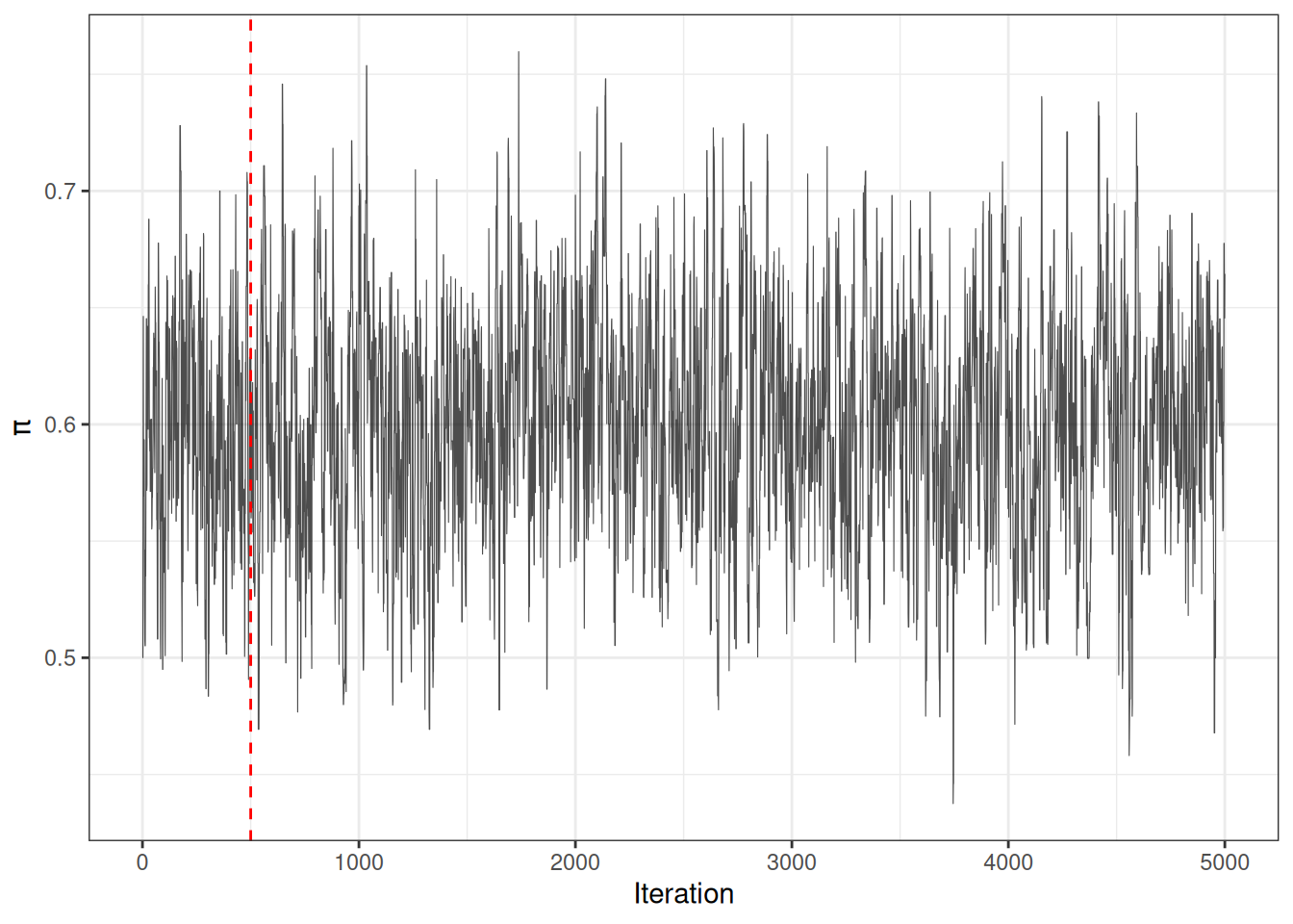
1.7.1 Trace plots

A trace plot graphs the sampled value \(\tilde{\theta}^{(t)}\) against iteration \(t\). A well-mixed chain shows rapid oscillation around a stable mean, with no obvious trends or stuck regions.

Exm

Example 3 (Trace plot for MH chain)

Show R code

burnin <- 500L
df_chain <- data.frame(iteration = seq_along(mh_chain), pi = mh_chain)
ggplot(df_chain, aes(x = iteration, y = pi)) +
  geom_line(linewidth = 0.2, alpha = 0.7) +
  geom_vline(xintercept = burnin, linetype = "dashed", colour = "red") +
  labs(x = "Iteration", y = expression(pi)) +
  theme_bw()

Figure 1: MH chain trace plot; dashed line marks end of burn-in.

1.7.2 Autocorrelation function (ACF)

Because successive draws in an MCMC chain are correlated, the effective sample size (ESS) is less than the number of iterations. The autocorrelation function (ACF) quantifies this dependence. A rapidly decaying ACF indicates good mixing.

1.7.3 Multiple chains and the Gelman–Rubin statistic

Running multiple chains from different starting points provides a stronger convergence check than a single chain. The Gelman–Rubin statistic \(\hat{R}\) compares within-chain and between-chain variance. \(\hat{R}\approx 1\) indicates convergence (Dobson and Barnett 2018, chap. 13, p. 304). A common rule of thumb is \(\hat{R}< 1.1\).

1.8 Posterior inference from MCMC samples

After discarding burn-in, the remaining chain \(\tilde{\theta}^{(B+1)}, \ldots, \tilde{\theta}^{(T)}\) is treated as a (correlated) sample from the posterior. Posterior summaries are computed as sample statistics:

Posterior mean: \(\hat{\mu}= \frac{1}{T - B} \sum_{t=B+1}^{T} \tilde{\theta}^{(t)}\)
Credible interval: sample quantiles of the chain after burn-in

(Dobson and Barnett 2018, chap. 13, p. 305).

Exm

Example 4 (Posterior summaries from MH chain) Using the chain from Example 2, we discard the first 500 iterations as burn-in and compute posterior summaries.

Show R code

burnin <- 500L
post_chain <- mh_chain[seq(burnin + 1L, length(mh_chain))]
round(c(
  mean  = mean(post_chain),
  lower = unname(quantile(post_chain, 0.025)),
  upper = unname(quantile(post_chain, 0.975))
), 4)
#>   mean  lower  upper 
#> 0.6014 0.5044 0.6958

2 Comparing MCMC estimates to maximum likelihood

It is reassuring — and a useful check — that for models where both approaches apply, the posterior mean from a well-mixed MCMC chain and the maximum likelihood estimate (MLE) typically agree closely when the prior is weak and the sample size is moderate or large (Dobson and Barnett 2018, chap. 13, p. 298). Intuitively, as \(n\) grows the likelihood dominates the prior, so the posterior concentrates near the MLE, and the posterior standard deviation approaches the frequentist standard error.

Exm

Example 5 (Posterior mean vs. MLE for a Bernoulli model) For the Beta-Bernoulli model with \(r = 55\) successes in \(n = 91\) trials, the MLE is \(\hat\pi = r/n\), while the posterior mean under a uniform prior is \((r+1)/(n+2)\). The two differ only by the prior’s pseudo-counts and converge as \(n\) grows:

Show R code

r_obs <- 55L
n_obs <- 91L
round(c(
  mle = r_obs / n_obs,
  posterior_mean = (r_obs + 1) / (n_obs + 2)
), 4)
#>            mle posterior_mean 
#>         0.6044         0.6022

A persistent discrepancy between the two, by contrast, is a signal worth investigating: it may reflect a genuinely informative prior, an unconverged chain, or a coding error in the model.

3 The importance of parameterization

How a model is written affects how well its sampler mixes (Dobson and Barnett 2018, chap. 13, p. 299). Two algebraically equivalent parameterizations of the same model can produce chains with very different autocorrelation: strong posterior correlation between parameters slows a component-wise sampler, because each update can only move one coordinate at a time along a narrow, tilted ridge.

Common remedies include centering predictors (subtracting their means) so that intercept and slope are less correlated, and reparameterizing variance components to a scale on which the posterior is more nearly symmetric. These changes leave the model’s likelihood and the scientific conclusions unchanged; they alter only the geometry the sampler must explore.

4 Bayesian model fit: the deviance information criterion

To compare competing Bayesian models we need a measure that balances goodness of fit against complexity, much as Akaike’s information criterion (AIC) does for likelihood-based models. The standard MCMC-based criterion is the deviance information criterion (DIC) (Dobson and Barnett 2018, chap. 13, p. 306).

Let \(D(\tilde{\theta}) = -2 \log p(\tilde{y}\mid \tilde{\theta})\) be the deviance. Write \(\overline{D}\) for its posterior mean (estimated by averaging \(D(\tilde{\theta}^{(t)})\) over the chain) and \(D(\bar{\tilde{\theta}})\) for the deviance evaluated at the posterior mean of the parameters.

Definition 4 (Deviance information criterion) The effective number of parameters and the DIC are

\[ \begin{aligned} p_D &\stackrel{\text{def}}{=}\overline{D} - D(\bar{\tilde{\theta}}),\\ \operatorname{DIC} &\stackrel{\text{def}}{=}D(\bar{\tilde{\theta}}) + 2\,p_D = \overline{D} + p_D. \end{aligned} \]

The term \(D(\bar{\tilde{\theta}})\) rewards fit, while \(p_D\) penalizes complexity: it measures how much the deviance is reduced, on average, by letting the parameters adapt to the data. As with AIC, lower DIC is better, and only differences in DIC between models fit to the same data are meaningful. Because \(p_D\) is computed directly from the posterior draws, DIC is a convenient by-product of an MCMC run; it should nonetheless be used with care, as it can behave poorly for models with weakly identified parameters or markedly non-normal posteriors.

References

Dobson, Annette J, and Adrian G Barnett. 2018. An Introduction to Generalized Linear Models. 4th ed. CRC press. https://doi.org/10.1201/9781315182780.