---
title: "Basic Statistical Methods"
format:
html: default
revealjs:
output-file: basic-statistical-methods-slides.html
pdf:
output-file: basic-statistical-methods-handout.pdf
docx:
output-file: basic-statistical-methods-handout.docx
---
{{< include shared-config.qmd >}}
## Acknowledgements {.unnumbered}
This content is adapted from @vittinghoff2e, Chapter 3.
# Introduction
This appendix reviews fundamental statistical methods
that are prerequisites for the main content of this course.
Most of this material should be familiar from Epi 202 and Epi 203.
---
## Example dataset: HERS {#sec-hers-intro .unnumbered}
Throughout this appendix we use the HERS dataset as a running example.
{{< include _subfiles/shared/_sec_hers_intro.qmd >}}
```{r}
#| eval: false
library(haven)
hers <- haven::read_dta(
  paste0(
    "https://regression.ucsf.edu/sites/g/files",
    "/tkssra6706/f/wysiwyg/home/data/hersdata.dta"
  )
)
```
```{r}
#| include: false
hers <- rmb::hers |> haven::zap_labels()
```
# Descriptive Statistics {#sec-descriptive-stats}
See @vittinghoff2e, §3.2.
## Summary statistics for continuous variables {#sec-summary-continuous}
### Sample mean
::: {#def-sample-mean}
#### Sample mean
The **sample mean** of $n$ observations $x_1, \ldots, x_n$ is:
$$\bar{x} = \frac{1}{n} \sum_{i=1}^{n} x_i$$
:::
### Sample variance
::: {#def-sample-variance}
#### Sample variance
The **sample variance** is:
$$s^2 = \frac{1}{n-1} \sum_{i=1}^{n} (x_i - \bar{x})^2$$
The divisor $n - 1$ (rather than $n$)
makes $s^2$ an [unbiased](estimation.qmd#def-unbiased) estimator
of the population variance $\sigma^2$.
:::
### Sample standard deviation
::: {#def-sample-sd}
#### Sample standard deviation
The **sample standard deviation** is $s = \sqrt{s^2}$.
It is expressed in the same units as the original data,
making it more interpretable than the variance.
:::
### Sample median
::: {#def-sample-median}
#### Sample median
The **sample median** is the middle value
when observations are sorted in ascending order.
For $n$ observations:
- If $n$ is odd, the median is the $\frac{n+1}{2}$th order statistic.
- If $n$ is even, the median is the average of the
$\frac{n}{2}$th and $\frac{n}{2}+1$th order statistics.
The median is more robust to outliers than the mean.
:::
### Interquartile range
::: {#def-IQR}
#### Interquartile range
The **interquartile range (IQR)** is the difference between the 75th percentile
(the third quartile, $Q_3$) and the 25th percentile
(the first quartile, $Q_1$):
$$\text{IQR} = Q_3 - Q_1$$
Like the median, the IQR is robust to outliers.
:::
## Summary statistics for categorical variables {#sec-summary-categorical}
### Sample proportion
::: {#def-sample-proportion}
#### Sample proportion
For a binary outcome,
the **sample proportion** of "successes" (coded as 1) is:
$$\hat{p} = \frac{k}{n}$$
where $k$ is the number of successes and $n$ is the total sample size.
:::
## Computing summary statistics in R {#sec-summary-R}
The `tbl_summary()` function from the `gtsummary` package
produces formatted summary tables:
### HERS baseline summary statistics
::: {#exm-hers-summary}
```{r}
#| label: tbl-hers-summary
#| code-fold: false
library(dplyr)
library(gtsummary)
library(haven)

hers |>
  mutate(
    HT = haven::as_factor(HT),
    exercise = haven::as_factor(exercise),
    smoking = haven::as_factor(smoking),
    diabetes = haven::as_factor(diabetes)
  ) |>
  select(age, BMI, glucose, SBP, DBP, HT, exercise, smoking, diabetes) |>
  tbl_summary(
    by = HT,
    statistic = list(
      gtsummary::all_continuous() ~ "{mean} ({sd})",
      gtsummary::all_categorical() ~ "{n} ({p}%)"
    ),
    digits = gtsummary::all_continuous() ~ 1,
    label = list(
      age ~ "Age (years)",
      BMI ~ "BMI (kg/m²)",
      glucose ~ "Fasting glucose (mg/dL)",
      SBP ~ "Systolic BP (mmHg)",
      DBP ~ "Diastolic BP (mmHg)",
      exercise ~ "Exercises regularly",
      smoking ~ "Current smoker",
      diabetes ~ "Diabetes"
    )
  ) |>
  add_overall() |>
  bold_labels()
```
:::
## Exploratory data analysis {#sec-eda}
Graphical summaries reveal aspects of the data distribution
that summary statistics may miss,
such as skewness, multimodality, and outliers.
### Histograms {#sec-histograms}
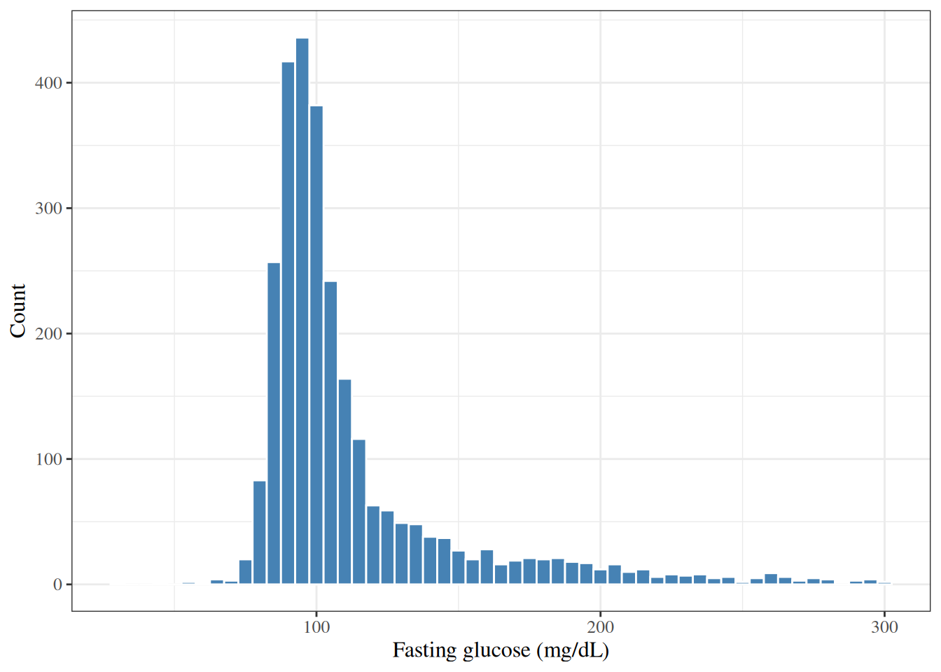
A **histogram** displays the distribution of a continuous variable
by dividing the range of values into intervals (bins)
and plotting the number or proportion of observations in each bin.
### Distribution of fasting glucose
::: {#exm-hers-histogram}
```{r}
#| label: fig-hers-histogram
#| fig-cap: "Distribution of fasting glucose (mg/dL) in HERS participants"
#| code-fold: false
library(ggplot2)

hers |>
  ggplot() +
  aes(x = glucose) +
  geom_histogram(binwidth = 5, fill = "steelblue", color = "white") +
  labs(
    x = "Fasting glucose (mg/dL)",
    y = "Count"
  )
```
:::
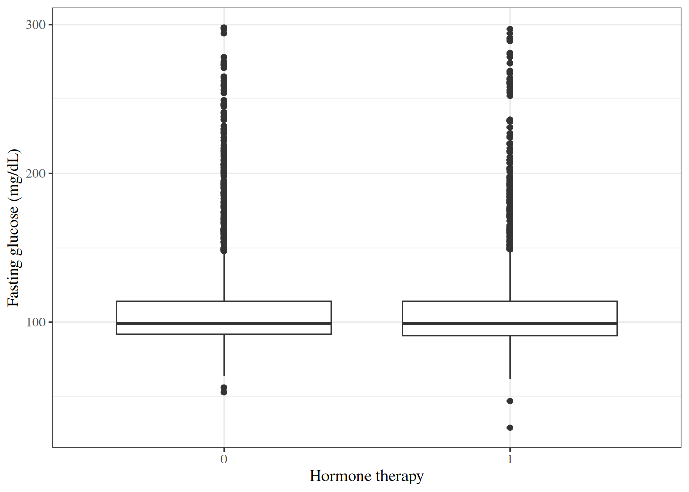
### Boxplots {#sec-boxplots}
A **boxplot** (box-and-whisker plot) summarizes the distribution of a continuous variable
using five statistics:
the minimum, the first quartile ($Q_1$),
the median, the third quartile ($Q_3$), and the maximum
(with outliers plotted separately).
### Fasting glucose by hormone therapy group
::: {#exm-hers-boxplot}
```{r}
#| label: fig-hers-boxplot
#| fig-cap: "Fasting glucose by hormone therapy assignment in HERS"
#| code-fold: false
hers |>
  mutate(HT = haven::as_factor(HT)) |>
  ggplot() +
  aes(x = HT, y = glucose) +
  geom_boxplot() +
  labs(
    x = "Hormone therapy",
    y = "Fasting glucose (mg/dL)"
  )
```
:::
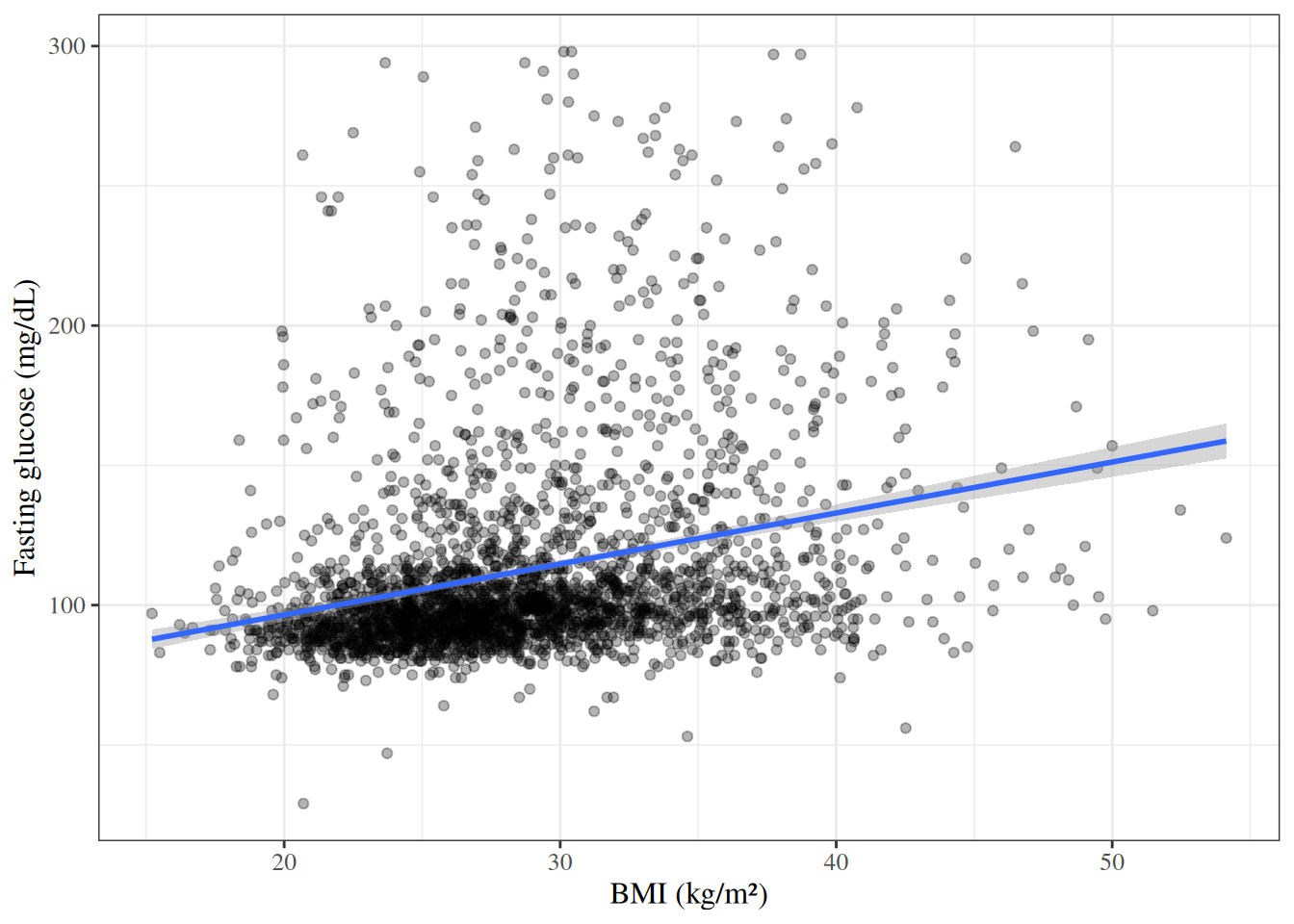
### Scatterplots {#sec-scatterplots}
A **scatterplot** displays the joint distribution of two continuous variables
by plotting each observation as a point.
### BMI versus fasting glucose
::: {#exm-hers-scatter}
```{r}
#| label: fig-hers-scatter
#| fig-cap: "Fasting glucose versus BMI in HERS participants"
#| code-fold: false
hers |>
  ggplot() +
  aes(x = BMI, y = glucose) +
  geom_point(alpha = 0.3) +
  geom_smooth(method = "lm", se = TRUE) +
  labs(
    x = "BMI (kg/m²)",
    y = "Fasting glucose (mg/dL)"
  )
```
:::
# Comparing Two Groups: Continuous Outcomes {#sec-two-group-continuous}
See @vittinghoff2e, §3.3.
## Hypotheses {#sec-hypotheses}
### Null hypothesis
::: {#def-null-hypothesis}
#### Null hypothesis
The **null hypothesis** $H_0$ is a specific claim
about the population parameter(s) that we test against the data.
In a two-group comparison of means,
the null hypothesis is typically that the two group means are equal:
$$H_0: \mu_1 = \mu_2$$
:::
### Alternative hypothesis
::: {#def-alternative-hypothesis}
#### Alternative hypothesis
The **alternative hypothesis** $H_1$ (or $H_A$) is the claim
we are trying to find evidence for.
For a two-sided test:
$$H_1: \mu_1 \neq \mu_2$$
:::
## The two-sample t-test {#sec-two-sample-t-test}
### Definition
::: {#def-two-sample-t-test}
#### Two-sample t-test
The **two-sample t-test** (Welch's t-test)
tests whether the means of two independent groups are equal.
For samples of sizes $n_1$ and $n_2$ from two groups
with sample means $\bar{x}_1$, $\bar{x}_2$
and sample variances $s_1^2$, $s_2^2$,
the test statistic is:
$$t = \frac{\bar{x}_1 - \bar{x}_2}{\sqrt{\dfrac{s_1^2}{n_1} + \dfrac{s_2^2}{n_2}}}$$
Under $H_0$, this statistic follows (approximately) a $t$-distribution
with degrees of freedom estimated by the Welch-Satterthwaite equation.
:::
### Welch's t-test vs. pooled t-test
::: callout-note
Welch's t-test (the default in R's `t.test()`)
does not assume equal variances across groups.
The pooled t-test assumes equal variances ($\sigma_1^2 = \sigma_2^2$)
and pools the two sample variances into a single estimate.
Welch's t-test is generally preferred
because the equal-variance assumption is rarely verifiable in practice
[@vittinghoff2e §3.3].
:::
### Comparing fasting glucose between hormone therapy groups
::: {#exm-hers-ttest}
We test $H_0: \mu_\text{placebo} = \mu_\text{HT}$
vs. $H_1: \mu_\text{placebo} \neq \mu_\text{HT}$.
```{r}
#| code-fold: false
glucose_placebo <- hers |> filter(HT == 0) |> pull(glucose)
glucose_HT <- hers |> filter(HT == 1) |> pull(glucose)
t.test(glucose_HT, glucose_placebo)
```
:::
## One-sample t-test {#sec-one-sample-t-test}
### Definition
::: {#def-one-sample-t-test}
#### One-sample t-test
The **one-sample t-test** tests whether the mean of a single population
equals a specified null value $\mu_0$:
$$H_0: \mu = \mu_0 \qquad H_1: \mu \neq \mu_0$$
The test statistic is:
$$t = \frac{\bar{x} - \mu_0}{s / \sqrt{n}}$$
Under $H_0$, $t \sim t_{n-1}$ (a t-distribution with $n-1$ degrees of freedom).
:::
## Paired t-test {#sec-paired-t-test}
### Definition
::: {#def-paired-t-test}
#### Paired t-test
The **paired t-test** compares two related measurements
(e.g., pre- and post-treatment values from the same subjects).
Let $d_i = x_{i,1} - x_{i,2}$ be the within-subject difference;
the test reduces to a one-sample t-test on the differences:
$$H_0: \mu_d = 0 \qquad H_1: \mu_d \neq 0$$
:::
### Change in glucose over follow-up
::: {#exm-hers-paired}
```{r}
#| code-fold: false
# glucose1 is follow-up glucose; glucose is baseline
t.test(hers$glucose1, hers$glucose, paired = TRUE)
```
:::
## Confidence intervals for the difference in means {#sec-CI-diff-means}
A two-sided $(1-\alpha) \cdot 100\%$ confidence interval
for $\mu_1 - \mu_2$ is:
$$(\bar{x}_1 - \bar{x}_2) \pm t^*_{df} \cdot \sqrt{\frac{s_1^2}{n_1} + \frac{s_2^2}{n_2}}$$
where $t^*_{df}$ is the appropriate critical value from the t-distribution.
The confidence interval is returned by `t.test()` in R
alongside the hypothesis test result.
For more on confidence intervals,
see [Statistical Inference](inference.qmd#sec-CI).
# One-Way Analysis of Variance {#sec-anova}
**Analysis of variance (ANOVA)** generalizes the two-sample t-test
to compare means across $k \geq 2$ groups.
## Definition
::: {#def-one-way-anova}
#### One-way ANOVA
In a **one-way ANOVA**, we test:
$$H_0: \mu_1 = \mu_2 = \cdots = \mu_k$$
vs. the alternative that at least one mean differs.
The F-statistic compares the **between-group variance**
to the **within-group variance**:
$$F = \frac{\text{MS}_\text{between}}{\text{MS}_\text{within}}
= \frac{\text{SS}_\text{between}/(k-1)}{\text{SS}_\text{within}/(n-k)}$$
Under $H_0$, $F \sim F_{k-1, n-k}$.
:::
### Fasting glucose by race/ethnicity
::: {#exm-hers-anova}
```{r}
#| code-fold: false
aov_result <- aov(glucose ~ factor(raceth), data = hers)
summary(aov_result)
```
:::
### ANOVA as a special case of linear regression
::: callout-note
One-way ANOVA is equivalent to a linear regression model
with a single categorical predictor.
See [Linear Models Overview](Linear-models-overview.qmd) for details.
:::
# Comparing Two Groups: Categorical Outcomes {#sec-two-group-categorical}
See @vittinghoff2e, §3.5.
## Contingency tables {#sec-contingency-tables}
### Definition
::: {#def-contingency-table}
#### Contingency table
A **contingency table** (cross-tabulation) displays
the joint frequencies of two categorical variables.
For two binary variables,
this is a $2 \times 2$ table with cells $a$, $b$, $c$, $d$:
| | Outcome = 1 | Outcome = 0 | Total |
|--------------------|:-----------:|:-----------:|:---------:|
| Exposure = 1 | $a$ | $b$ | $a + b$ |
| Exposure = 0 | $c$ | $d$ | $c + d$ |
| Total | $a + c$ | $b + d$ | $n$ |
:::
### Exercise by hormone therapy group
::: {#exm-hers-crosstab}
```{r}
#| label: tbl-hers-crosstab
#| tbl-cap: "Exercise by hormone therapy group in HERS"
#| code-fold: false
hers |>
  mutate(
    HT = haven::as_factor(HT),
    exercise = haven::as_factor(exercise)
  ) |>
  gtsummary::tbl_cross(
    row = exercise,
    col = HT,
    label = list(
      exercise ~ "Exercises regularly",
      HT ~ "Hormone therapy"
    ),
    percent = "row"
  )
```
:::
## The chi-square test {#sec-chi-square}
### Definition
::: {#def-chi-square-test}
#### Chi-square test
The **Pearson chi-square test** tests whether two categorical variables are independent.
For a $2 \times 2$ table,
the test statistic is:
$$\chi^2 = \sum_{i,j} \frac{(O_{ij} - E_{ij})^2}{E_{ij}}$$
where $O_{ij}$ is the observed cell count
and $E_{ij} = \frac{(\text{row total}) \times (\text{column total})}{n}$
is the expected cell count under independence.
Under $H_0$ (independence), $\chi^2 \sim \chi^2_1$
for a $2 \times 2$ table.
:::
### Chi-square test: exercise vs. hormone therapy
::: {#exm-hers-chisq}
```{r}
#| code-fold: false
chisq.test(hers$exercise, hers$HT)
```
:::
## Fisher's exact test {#sec-fisher}
### Definition
::: {#def-fishers-exact}
#### Fisher's exact test
**Fisher's exact test** computes the exact probability of observing
a $2 \times 2$ table at least as extreme as the observed table,
given the marginal totals and under the null hypothesis of independence.
It is preferred over the chi-square test when cell counts are small
(typically when any expected cell count is less than 5).
:::
### Fisher's exact test example
::: {#exm-hers-fisher}
```{r}
#| code-fold: false
fisher.test(hers$exercise, hers$HT)
```
:::
## Measures of association for 2×2 tables {#sec-2x2-measures}
See [Odds Ratios and Relative Risks](logistic-regression.qmd#sec-OR-RR) for definitions and formulas.
# Correlation {#sec-correlation}
See @vittinghoff2e, §3.6.
## Pearson correlation coefficient {#sec-pearson}
### Definition
::: {#def-pearson-r}
#### Pearson correlation coefficient
The **Pearson correlation coefficient** measures the strength and direction
of the linear association between two continuous variables $X$ and $Y$:
$$r = \frac{\sum_{i=1}^{n} (x_i - \bar{x})(y_i - \bar{y})}
{\sqrt{\sum_{i=1}^{n}(x_i - \bar{x})^2 \sum_{i=1}^{n}(y_i - \bar{y})^2}}$$
$r$ ranges from $-1$ (perfect negative linear relationship) to $+1$
(perfect positive linear relationship);
$r = 0$ indicates no linear association.
:::
### Correlation between BMI and glucose
::: {#exm-hers-cor}
```{r}
#| code-fold: false
cor.test(hers$BMI, hers$glucose, method = "pearson")
```
:::
## Spearman rank correlation {#sec-spearman}
### Definition
::: {#def-spearman-r}
#### Spearman rank correlation
The **Spearman rank correlation** $r_S$
is the Pearson correlation computed on the *ranks* of the observations.
It measures the strength and direction of any *monotone* association
(not just linear) and is more robust to outliers.
:::
### Spearman correlation between BMI and glucose
::: {#exm-hers-spearman}
```{r}
#| code-fold: false
cor.test(hers$BMI, hers$glucose, method = "spearman")
```
:::
# Simple Linear Regression {#sec-simple-linear-regression}
See @vittinghoff2e, §3.6 and [Linear Models Overview](Linear-models-overview.qmd).
## Model specification {#sec-slr-model}
### Definition
::: {#def-slr}
#### Simple linear regression
A **simple linear regression** model relates
a continuous outcome $Y$ to a single predictor $X$:
$$Y_i = \b_0 + \b_1 x_i + \varepsilon_i, \qquad \varepsilon_i \overset{\text{iid}}{\sim} \ndist{0, \sigma^2}$$
- $\b_0$ is the **intercept**:
the expected value of $Y$ when $X = 0$.
- $\b_1$ is the **slope**:
the expected change in $Y$ per one-unit increase in $X$.
- $\varepsilon_i$ are independent Gaussian errors with mean 0 and variance $\sigma^2$.
:::
## Ordinary least squares estimation {#sec-ols}
The parameters $\b_0$ and $\b_1$ are estimated
by minimizing the **residual sum of squares (RSS)**:
$$\text{RSS} = \sum_{i=1}^n (y_i - \hat{y}_i)^2
= \sum_{i=1}^n (y_i - \hat\b_0 - \hat\b_1 x_i)^2$$
The closed-form **ordinary least squares (OLS)** estimators are:
$$\hat\b_1 = r \cdot \frac{s_y}{s_x}, \qquad \hat\b_0 = \bar{y} - \hat\b_1 \bar{x}$$
where $r$ is the Pearson correlation and $s_x$, $s_y$ are the sample standard deviations.
## Fitting a simple linear regression in R {#sec-slr-R}
### Glucose on BMI
::: {#exm-hers-slr}
```{r}
#| label: tbl-hers-slr
#| code-fold: false
slr_fit <- lm(glucose ~ BMI, data = hers)
summary(slr_fit)
```
The estimated slope is
$\hat\b_1 = `r round(coef(slr_fit)[["BMI"]], 2)`$ mg/dL per kg/m²,
meaning fasting glucose increases by approximately
`r round(coef(slr_fit)[["BMI"]], 2)` mg/dL
for each 1 kg/m² increase in BMI.
:::
## The coefficient of determination ($R^2$) {#sec-r-squared}
### Definition
::: {#def-r-squared}
#### Coefficient of determination ($R^2$)
The **coefficient of determination** $R^2$ measures the proportion of the total
variance in $Y$ that is explained by the linear regression on $X$:
$$R^2 = 1 - \frac{\text{RSS}}{\text{TSS}}
= 1 - \frac{\sum_i (y_i - \hat{y}_i)^2}{\sum_i (y_i - \bar{y})^2}$$
$R^2$ ranges from 0 (no linear relationship)
to 1 (perfect linear fit).
For simple linear regression, $R^2 = r^2$.
:::
## Further reading
For a more thorough treatment of linear regression,
see [Linear Models Overview](Linear-models-overview.qmd)
and @vittinghoff2e, Chapters 4 and 9.
# Bootstrap Confidence Intervals {#sec-bootstrap-ci}
::: notes
Adapted from
[@vittinghoff2e, Section 3.6, pp. 62–63].
:::
## When to use the bootstrap {#sec-bootstrap-when}
Bootstrapping is a widely applicable method
for obtaining standard errors and CIs
in three situations:
- Approximate methods for computing valid CIs have been developed
but are not conveniently implemented in standard software.
- Developing closed-form approximate methods has turned out to be intractable.
- The dataset violates the assumptions underlying established methods badly enough
that the resulting CIs would be unreliable.
## The bootstrap procedure {#sec-bootstrap-procedure}
::: {#def-bootstrap-sample}
#### Bootstrap sample
A **bootstrap sample** is a sample of size $n$
drawn **with replacement** from the observed data of size $n$.
Because sampling is with replacement,
each bootstrap sample contains some observations more than once
and omits others entirely.
:::
::: {#exm-bootstrap-sample-toy}
#### Bootstrap sample
Consider a dataset of five observations: $\{3,\;7,\;5,\;2,\;9\}$ ($n = 5$).
Two possible bootstrap samples drawn with replacement are:
| Bootstrap sample | Values drawn | Notes |
|:---:|:---:|:---|
| 1 | $3,\;3,\;7,\;5,\;9$ | 3 appears twice; 2 not drawn |
| 2 | $2,\;7,\;7,\;9,\;5$ | 7 appears twice; 3 not drawn |
Each sample has size $n = 5$
but may repeat or omit individual observations from the original dataset.
:::
::: {#def-bootstrap-distribution}
#### Bootstrap distribution
The **bootstrap distribution** of a statistic
is the empirical distribution of that statistic
computed across a large number $B$ of bootstrap samples.
It serves as an estimate of the sampling distribution of the statistic.
The **bootstrap standard error** is the standard deviation
of the bootstrap distribution.
:::
::: {#exm-bootstrap-distribution-toy}
#### Bootstrap distribution
```{r}
#| label: setup-boot-dist-toy
set.seed(42)
toy <- c(3, 7, 5, 2, 9, 4, 8, 1, 6, 10)
boot_means_toy <- replicate(
  1000,
  mean(sample(toy, replace = TRUE))
)
boot_se_toy <- sd(boot_means_toy)
boot_ci_norm_lo <- mean(toy) - 1.96 * boot_se_toy
boot_ci_norm_hi <- mean(toy) + 1.96 * boot_se_toy
boot_ci_perc <- quantile(boot_means_toy, c(0.025, 0.975))
```
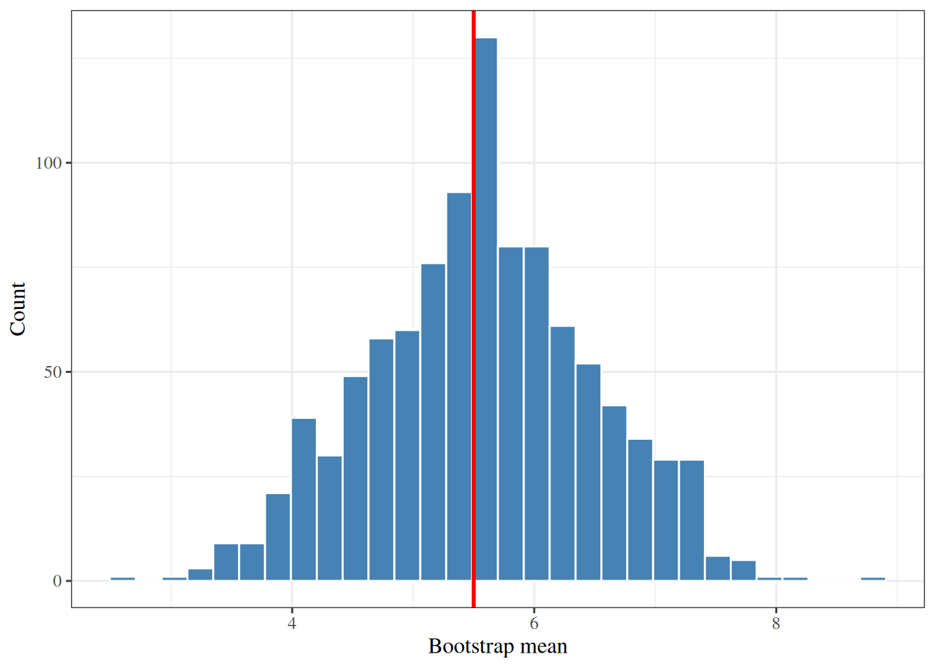
Using the 10-observation dataset $\cb{3, 7, 5, 2, 9, 4, 8, 1, 6, 10}$
(observed mean `r mean(toy)`),
we draw $B = 1{,}000$ bootstrap resamples
and compute the sample mean of each.
The bootstrap distribution is centered near the observed mean
with bootstrap standard error `r round(boot_se_toy, 2)`.
::: {#fig-boot-dist-toy}
```{r}
#| code-fold: true
library(ggplot2)
ggplot(data.frame(mean = boot_means_toy)) +
  aes(x = mean) +
  geom_histogram(bins = 30, color = "white", fill = "steelblue") +
  geom_vline(xintercept = mean(toy), color = "red", linewidth = 1) +
  labs(x = "Bootstrap mean", y = "Count")
```
Bootstrap distribution of the sample mean
($B = 1{,}000$ replicates, $n = 10$ toy dataset).
The red line marks the observed mean (`r mean(toy)`).
The distribution is approximately normal and centered near $\bar{x}$.
:::
:::
The key idea is to treat the observed sample as a stand-in
for the source population,
and to mimic repeated sampling from that population
by resampling with replacement from the observed data.
## Bootstrap CI methods {#sec-bootstrap-methods}
Three methods for constructing a CI from the bootstrap distribution
are in common use
[@vittinghoff2e, Section 3.6, p. 63]:
### Normal approximation {#sec-bootstrap-normal}
If the bootstrap distribution of the statistic of interest
is approximately normal,
replace the model-based standard error in a conventional CI
with the bootstrap standard deviation:
$$\hat\theta \pm z^* \cdot \widehat{\text{SE}}_{\text{boot}}$$
This method requires fewer bootstrap replicates than percentile-based methods,
but is less reliable when the sampling distribution departs from normality,
particularly in the tails.
::: {#exm-bootstrap-normal-toy}
#### Normal approximation
Continuing from @exm-bootstrap-distribution-toy:
the observed mean is `r mean(toy)`
and the bootstrap standard error is `r round(boot_se_toy, 2)`.
The 95% normal-approximation CI is:
$$\bar{x} \pm 1.96 \cdot \widehat{\text{SE}}_{\text{boot}}$$
which here evaluates to
(`r round(boot_ci_norm_lo, 2)`, `r round(boot_ci_norm_hi, 2)`).
:::
### Percentile method {#sec-bootstrap-percentile}
The CI is constructed from the empirical quantiles of the bootstrap distribution.
A 95% CI spans the 2.5th to 97.5th percentiles
of the $B$ bootstrap estimates.
Because the extreme percentiles of a finite sample are noisy estimates
of the corresponding population quantiles,
a larger number of replicates is required
(typically $B \geq 1{,}000$).
::: {#exm-bootstrap-percentile-toy}
#### Percentile method
Continuing from @exm-bootstrap-distribution-toy
with $B = 1{,}000$ bootstrap means:
the 2.5th percentile is `r round(boot_ci_perc[[1]], 2)`
and the 97.5th percentile is `r round(boot_ci_perc[[2]], 2)`,
giving a 95% CI of
(`r round(boot_ci_perc[[1]], 2)`, `r round(boot_ci_perc[[2]], 2)`).
:::
### Bias-corrected and accelerated (BCa) method {#sec-bootstrap-bca}
The BCa interval adjusts the percentile-based CI
to account for both bias
(a shift between the observed statistic and the median of the bootstrap distribution)
and skewness in the bootstrap distribution
[@james2021islr2e, Chapter 5, p. 209].
BCa intervals are preferred when the bootstrap distribution is noticeably skewed.
::: {#exm-bootstrap-bca-toy}
#### Bias-corrected and accelerated method
The BCa interval for the toy dataset is computed automatically
by `boot.ci()` in R,
which handles the bias-correction and acceleration adjustments internally.
The comprehensive worked example below
demonstrates all three CI methods side by side,
making it straightforward to compare the BCa interval
to the normal and percentile intervals.
:::
## Bootstrap CI in R {#sec-bootstrap-R}
The `boot` package (included with base R) provides
`boot()` for resampling and `boot.ci()` for all three CI types.
### Bootstrap CI for the slope of SBP on age {#sec-bootstrap-hers}
::: {#exm-hers-bootstrap}
We adapt the example from
[@vittinghoff2e, Section 3.6, p. 62]:
a simple linear regression of systolic blood pressure (`SBP`) on `age`
in the HERS dataset.
```{r}
#| label: exm-bootstrap-sbp-age
#| code-fold: true
library(boot)
# statistic function: returns the slope of SBP ~ age
boot_slope <- function(data, indices) {
fit <- lm(SBP ~ age, data = data[indices, ])
coef(fit)[["age"]]
}
set.seed(42)
boot_result <- boot(
data = hers,
statistic = boot_slope,
R = 1000
)
boot_result
```
The bootstrap standard error closely matches
the model-based standard error from `lm()`.
All three bootstrap intervals below are consistent with the parametric CI.
```{r}
#| label: exm-bootstrap-sbp-age-ci
#| code-fold: true
boot.ci(
boot_result,
type = c("norm", "perc", "bca")
)
```
The normal, percentile, and BCa intervals are all similar here,
consistent with the bootstrap distribution being approximately symmetric.
In cases with more skewness,
the BCa interval would differ more from the others,
and should be preferred.
:::