---
title: "Bayesian Analysis"
format:
html: default
revealjs:
output-file: intro-bayes-slides.html
pdf:
output-file: intro-bayes-handout.pdf
docx:
output-file: intro-bayes-handout.docx
---
{{< include shared-config.qmd >}}
This appendix introduces the **Bayesian** approach to statistical inference.
The structure parallels the development in [@dobson4e, Chapter 12]:
we contrast the frequentist and Bayesian paradigms,
state Bayes' theorem as an inference rule for parameters,
discuss the role of the prior distribution,
and outline hierarchical models and the software used to fit them.
Computation by simulation is deferred to
[the next appendix](mcmc-methods.qmd#sec-mcmc-methods),
and fully worked analyses appear in
[the appendix of example analyses](bayesian-examples.qmd#sec-bayes-examples).
# Frequentist and Bayesian paradigms {#sec-bayes-paradigms}
Throughout these notes we have treated an unknown parameter $\theta$
as a fixed but unknown constant,
and we have quantified uncertainty using the sampling distribution
of an estimator $\hat\theta$ —
that is, the distribution of $\hat\theta$ over hypothetical repetitions
of the data-generating process.
This stance is the **frequentist** paradigm:
probability describes long-run frequencies,
and a parameter, being a constant, has no probability distribution.
The **Bayesian** paradigm instead treats the unknown parameter as a
**random variable** with its own probability distribution
[@dobson4e, Chapter 12, p. 271].
Probability here measures *degree of belief*:
before seeing data we encode our uncertainty about $\theta$ in a
**prior distribution** $p(\theta)$,
and after observing data $\vy$ we update that belief to a
**posterior distribution** $p(\theta \mid \vy)$.
All Bayesian inference flows from this single posterior distribution.
::: notes
The two paradigms answer subtly different questions.
A frequentist asks, "for what parameter values would these data be
unsurprising?"; a Bayesian asks, "given these data, what should I now
believe about the parameter?".
Neither question is wrong; they are different, and they call for
different machinery.
:::
## Two readings of an interval estimate {#sec-bayes-interval-interp}
The distinction is sharpest in how each paradigm interprets an interval
estimate [@dobson4e, Chapter 12, p. 271].
A frequentist $95\%$ **confidence interval** $\paren{l(\vy),\, r(\vy)}$
is a random interval whose *coverage* —
the probability, over repeated sampling, that the interval contains the
fixed true $\theta$ — is $0.95$.
For one realized data set the interval either contains $\theta$ or it
does not; the $0.95$ refers to the procedure, not to the particular
interval.
A Bayesian **credible interval** makes the statement many users
*want* to make about a confidence interval but cannot:
:::{#def-credible-interval}
#### Credible interval
A $100(1-\alpha)\%$ **credible interval** for $\theta$ is an interval
$\paren{l(\vy),\, r(\vy)}$ such that, under the posterior distribution,
$$
p\sb{l(\vy) \le \theta \le r(\vy) \mid \vy} \eqdef 1 - \alpha.
$$
:::
Here the data $\vy$ are fixed at their observed values and $\theta$ is
random, so the probability statement is about $\theta$ directly.
# Bayes' theorem for parameters {#sec-bayes-equation}
The engine of Bayesian inference is **Bayes' theorem**,
applied to the parameter and the data.
Writing $p(\theta)$ for the prior and $\Lik(\theta) = p(\vy \mid \theta)$
for the likelihood,
the posterior is
:::{#def-posterior}
#### Posterior distribution
$$
p(\theta \mid \vy)
\eqdef
\frac{p(\vy \mid \theta)\,p(\theta)}{p(\vy)},
\qquad
p(\vy) = \int p(\vy \mid \theta)\,p(\theta)\,d\theta.
$$ {#eq-bayes-posterior}
:::
The denominator $p(\vy)$ — the **marginal likelihood** or
*evidence* — does not depend on $\theta$;
it is the constant that makes the posterior integrate to one.
Consequently the posterior is determined up to proportionality by the
numerator alone [@dobson4e, Chapter 12, p. 272]:
$$
\underbrace{p(\theta \mid \vy)}_{\text{posterior}}
\;\propto\;
\underbrace{p(\vy \mid \theta)}_{\text{likelihood}}
\cdot
\underbrace{p(\theta)}_{\text{prior}}.
$$ {#eq-bayes-proportional}
This proportionality is the workhorse of applied Bayesian analysis:
it lets us recognize the posterior from the shape of
$\text{likelihood} \times \text{prior}$ without ever computing the
integral $p(\vy)$, and it is what makes the simulation methods of
[the next appendix](mcmc-methods.qmd#sec-mcmc-methods) possible.
## A Gaussian mean with a Gaussian prior {#sec-bayes-normal-normal}
When prior and likelihood combine to give a posterior in the same family
as the prior, the prior is called **conjugate**.
The normal-mean model is the cleanest example.
:::{#exm-normal-normal}
#### Posterior for a normal mean
Suppose $X_1, \ldots, X_n \siid \ndist{\mu, 1}$ with the variance known,
and place a $\ndist{0, 1}$ prior on the mean: $M \sim \ndist{0, 1}$.
Collecting the terms of $p(M = \mu \mid X = x) \propto p(X = x \mid M = \mu)\,p(M = \mu)$
that involve $\mu$ and completing the square:
$$
\ba
p(M=\mu \mid X=x)
&\propto p(X=x \mid M=\mu)\, p(M=\mu)\\
&\propto \expf{-\frac{1}{2}\paren{n\mu^2 - 2\mu n\bar{x}}}
\cdot \expf{-\frac{1}{2}\mu^2}\\
&= \expf{-\frac{1}{2}\paren{(n+1)\mu^2 - 2\mu n\bar{x}}}\\
&\propto \expf{-\frac{1}{2}(n+1)\paren{\mu - \frac{n}{n+1}\bar{x}}^2}.
\ea
$$
The last line is the kernel of a normal density, so the posterior is
$$
M \mid X = x \;\sim\; \ndist{\frac{n}{n+1}\bar{x},\; \frac{1}{n+1}}.
$$
The posterior mean $\frac{n}{n+1}\bar{x}$ is the sample mean shrunk
toward the prior mean $0$, and the shrinkage vanishes as $n \to \infty$.
:::
# The parameter space {#sec-bayes-parameter-space}
Because the Bayesian treats $\theta$ as random, the prior and posterior
are distributions over the **parameter space** $\Theta$ —
the set of values $\theta$ can take
[@dobson4e, Chapter 12, p. 274].
The parameter space must be respected when choosing a prior:
a probability $\pi \in (0,1)$ calls for a prior supported on the unit
interval (such as a Beta distribution),
a variance $\sigma^2 > 0$ calls for a prior on the positive half-line,
and a vector of regression coefficients calls for a multivariate prior
on $\reals^p$.
A prior that places no mass on part of $\Theta$ forces the posterior to
do the same, no matter what the data say —
so the support of the prior is itself a modeling assumption.
:::{#exm-normal-credible-vs-confidence}
#### Credible vs. confidence interval for a normal mean
We compare the two interval estimates from @sec-bayes-interval-interp on
simulated data from the model of @exm-normal-normal.
First, the frequentist interval:
```{r}
set.seed(1)
mu <- 2
sigma <- 1
n <- 20
x <- rnorm(n = n, mean = mu, sd = sigma)
xbar <- mean(x)
se <- sigma / sqrt(n)
CI_freq <- xbar + se * qnorm(c(.025, .975))
print(CI_freq)
```
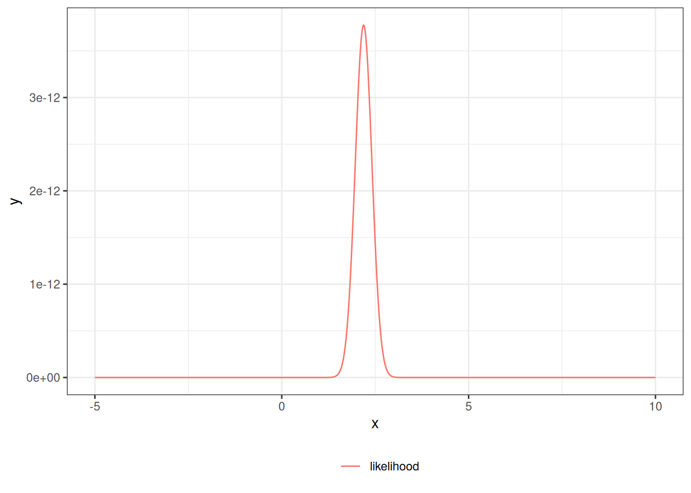
The likelihood as a function of $\mu$:
```{r}
lik <- function(mu) {
  (2 * pi * sigma^2)^(-n / 2) *
    exp(
      -1 / (2 * sigma^2) *
        (sum(x^2) - 2 * mu * sum(x) + n * (mu^2))
    )
}
library(ggplot2)
ngraph <- 1001
plot1 <- ggplot() +
  geom_function(fun = lik, aes(col = "likelihood"), n = ngraph) +
  xlim(c(-5, 10)) +
  theme_bw() +
  labs(col = "") +
  theme(legend.position = "bottom")
print(plot1)
```
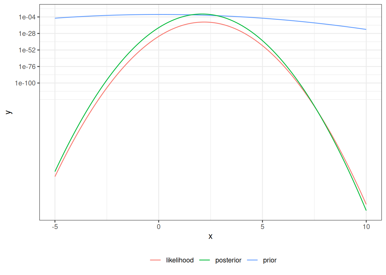
Next, the Bayesian credible interval, using the closed-form posterior
$\ndist{\frac{n}{n+1}\bar{x},\, (n+1)^{-1}}$ from @exm-normal-normal:
```{r}
mu_prior_mean <- 0
mu_prior_sd <- 1
mu_post_mean <- n / (n + 1) * xbar
mu_post_var <- 1 / (n + 1)
mu_post_sd <- sqrt(mu_post_var)
CI_bayes <- qnorm(
p = c(.025, .975),
mean = mu_post_mean,
sd = mu_post_sd
)
print(CI_bayes)
prior <- function(mu) dnorm(mu, mean = mu_prior_mean, sd = mu_prior_sd)
posterior <- function(mu) dnorm(mu, mean = mu_post_mean, sd = mu_post_sd)
plot2 <- plot1 +
geom_function(fun = prior, aes(col = "prior"), n = ngraph) +
geom_function(fun = posterior, aes(col = "posterior"), n = ngraph)
print(plot2 + scale_y_log10())
```
Finally, the quantity a credible interval reports —
the posterior probability that $M$ lies in the *frequentist* interval —
is well defined for the Bayesian but not for the frequentist:
```{r}
pr_in_CI <- pnorm(
CI_freq,
mean = mu_post_mean,
sd = mu_post_sd
) |> diff()
print(pr_in_CI)
```
:::
# Priors {#sec-bayes-priors}
The prior distribution $p(\theta)$ encodes what is known about
$\theta$ before the current data are seen.
Choosing it is the step that most distinguishes Bayesian practice from
frequentist practice, and it is where most of the controversy and most
of the craft live [@dobson4e, Chapter 12, p. 281].
## Conjugate priors {#sec-bayes-conjugate}
A prior is **conjugate** to a likelihood when the resulting posterior
belongs to the same parametric family as the prior.
Conjugate priors make the posterior available in closed form, as in
@exm-normal-normal.
The Beta family is conjugate to the Bernoulli/binomial likelihood:
:::{#exm-beta-bernoulli}
#### Beta-Bernoulli updating
Let $Y_1, \ldots, Y_n \siid \Bernoulli(\pi)$ with $r = \sum_i y_i$
successes, and place a $\operatorname{Beta}(a, b)$ prior on $\pi$.
By @eq-bayes-proportional,
$$
p(\pi \mid \vy)
\propto \underbrace{\pi^{r}(1-\pi)^{n-r}}_{\text{likelihood}}
\cdot \underbrace{\pi^{a-1}(1-\pi)^{b-1}}_{\text{prior}}
= \pi^{a + r - 1}(1-\pi)^{b + n - r - 1},
$$
which is the kernel of a $\operatorname{Beta}(a + r,\; b + n - r)$ density.
The prior parameters $a$ and $b$ act as **pseudo-counts** of prior
successes and failures: the posterior simply adds the observed $r$
successes and $n - r$ failures to them.
With a uniform $\operatorname{Beta}(1, 1)$ prior, $n = 91$, and $r = 55$,
the posterior is $\operatorname{Beta}(56, 37)$:
```{r}
a_prior <- 1
b_prior <- 1
n_obs <- 91
r_obs <- 55
a_post <- a_prior + r_obs
b_post <- b_prior + n_obs - r_obs
round(c(
post_mean = a_post / (a_post + b_post),
post_lower = qbeta(0.025, a_post, b_post),
post_upper = qbeta(0.975, a_post, b_post)
), 4)
```
:::
## Informative, weakly informative, and flat priors {#sec-bayes-informativeness}
Priors range along a spectrum of how much they constrain $\theta$
[@dobson4e, Chapter 12, p. 281]:
- An **informative** prior concentrates mass in a region supported by
external knowledge (previous studies, biological limits, expert
judgment). It pulls the posterior toward that region, most strongly
when the data are sparse.
- A **weakly informative** prior rules out implausible values
(for example, an odds ratio of $10^6$) while remaining flat across the
range of scientifically plausible values.
- A **flat** (or **noninformative**) prior aims to "let the data speak,"
approximating constant density over $\Theta$. Flat priors can be
*improper* (not integrating to one) and are not invariant to
reparameterization, so they require care.
## A skeptical prior {#sec-bayes-skeptical}
A useful special case is a **skeptical prior**, centered on "no effect"
and deliberately tight, used to ask how strong the data must be to
overturn a default of no effect [@dobson4e, Chapter 12, p. 281].
:::{#exm-skeptical-prior}
#### A skeptical prior for a normal mean
Reusing the normal-mean model of @exm-normal-normal but with a skeptical
$\ndist{0, \tau^2}$ prior of standard deviation $\tau$,
the posterior mean is the precision-weighted average
$$
\E{M \mid X = x}
= \frac{n\,\bar{x}}{n + 1/\tau^2},
$$
which shrinks toward $0$ more aggressively as the prior becomes more
skeptical (smaller $\tau$). We tabulate the posterior mean across a range
of prior skepticism, holding the data fixed:
```{r}
xbar_obs <- 2
n_obs2 <- 20
tau_grid <- c(0.1, 0.25, 0.5, 1, 2, 10)
post_mean <- (n_obs2 * xbar_obs) / (n_obs2 + 1 / tau_grid^2)
round(
  data.frame(prior_sd = tau_grid, posterior_mean = post_mean),
  3
)
```
A very skeptical prior ($\tau = 0.1$) drags the posterior mean almost to
zero despite $\bar{x} = 2$; a diffuse prior ($\tau = 10$) leaves it
essentially at the sample mean.
:::
# Distributions and hierarchies {#sec-bayes-hierarchies}
Many models have parameters that are themselves naturally described by a
distribution with further unknown parameters
[@dobson4e, Chapter 12, p. 281].
A **hierarchical** (or **multilevel**) model builds the prior in stages:
a **hyperprior** governs **hyperparameters**, which govern the
group-level parameters, which govern the data.
For example, with groups $j = 1, \ldots, J$,
each with its own mean $\theta_j$,
a two-level model might specify
$$
\ba
Y_{ij} \mid \theta_j &\sim \ndist{\theta_j,\, \sigma^2},\\
\theta_j \mid \mu, \tau &\sim \ndist{\mu,\, \tau^2},\\
\mu, \tau &\sim \text{hyperprior}.
\ea
$$
The middle level lets the groups **borrow strength** from one another:
the posterior for each $\theta_j$ is pulled toward the overall mean
$\mu$, by an amount governed by the between-group spread $\tau$ that the
data themselves estimate.
This is the Bayesian counterpart of the random-effects models of
[@dobson4e, Chapter 11];
[the random-effects example](bayesian-examples.qmd#sec-bayes-examples-random-effects)
fits one by simulation.
# Software for Bayesian computation {#sec-bayes-software}
Outside conjugate special cases, the posterior rarely has a closed form,
and the normalizing constant $p(\vy)$ in @eq-bayes-posterior is an
intractable integral.
Practical Bayesian analysis therefore relies on simulation —
**Markov chain Monte Carlo (MCMC)** — implemented in dedicated software
[@dobson4e, Chapter 12, p. 281].
The Dobson and Barnett text uses WinBUGS;
in these notes we use **JAGS** ("Just Another Gibbs Sampler") through R,
which follows the same model-specification style.
Related tools include **Stan** (Hamiltonian Monte Carlo) and the R
package **`brms`**, which compiles familiar formula syntax to Stan.
The mechanics of MCMC — why it is needed, how the samplers work, and how
to check that they have converged — are the subject of
[the next appendix](mcmc-methods.qmd#sec-mcmc-methods).
Worked analyses of real data sets follow in
[the appendix of example analyses](bayesian-examples.qmd#sec-bayes-examples).
# References {.unnumbered}
::: {#refs}
:::