---
title: "Predictor Selection"
subtitle: "Choosing which variables to include in a regression model"
format:
html: default
revealjs:
output-file: predictor-selection-slides.html
pdf:
output-file: predictor-selection-handout.pdf
---
{{< include shared-config.qmd >}}
# Acknowledgements {.unnumbered}
This content is adapted from:
- [@vittinghoff2e, Chapter 10]
- [@heinze2018variable]
# Introduction {#sec-pred-sel-intro}
{{< include _sec-pred-sel-overview.qmd >}}
# Inferential Goals {#sec-pred-sel-goals-chapter}
{{< include _sec-pred-sel-goals.qmd >}}
# Causal Thinking and DAGs {#sec-pred-sel-causal}
{{< include _sec-pred-sel-dag.qmd >}}
# Prediction {#sec-pred-sel-prediction}
{{< include _sec-pred-sel-prediction.qmd >}}
# Evaluating a Predictor of Primary Interest {#sec-pred-sel-eval}
{{< include _sec-pred-sel-primary.qmd >}}
# Identifying Multiple Important Predictors {#sec-pred-sel-multiple-chapter}
{{< include _sec-pred-sel-multiple.qmd >}}
# Testing-based selection {#sec-pred-sel-stepwise}
::: notes
Testing-based selection methods use statistical tests
(such as F-tests or likelihood ratio tests)
to decide which predictors to include in a model.
:::
## Stepwise regression
::: {.callout-warning}
## Caution about stepwise selection
Stepwise regression has well-known problems:
- It tends to select too many variables (overfitting).
- P-values and confidence intervals are biased after selection.
- It ignores model uncertainty.
- Results can be unstable across different samples.
Consider using subject-matter knowledge (DAGs),
cross-validation, or penalized methods (such as LASSO) instead.
See @heinze2018variable for a thorough review.
:::
The basic idea of stepwise selection:
- **Forward selection**: Start with no predictors;
add the predictor that most improves model fit at each step.
- **Backward elimination**: Start with all predictors;
remove the predictor that least worsens model fit at each step.
- **Bidirectional stepwise**: Combine forward and backward steps.
## Example: stepwise selection for LDL
```{r}
#| label: stepwise-ldl
# Full model with all candidate predictors
full_model_ldl <- lm(
LDL ~ HT + age + BMI + diabetes + smoking + statins + SBP,
data = hers_ldl
)
# Backward elimination using AIC
step_model_ldl <- step(
full_model_ldl,
direction = "backward",
trace = 0
)
summary(step_model_ldl)
```
# Criterion-based selection {#sec-pred-sel-aic-bic}
## AIC and BIC
When comparing non-nested models,
we can use information criteria:
- **AIC** (Akaike Information Criterion):
$$\text{AIC} = -2\,\hat\ell + 2p$$
- **BIC** (Bayesian Information Criterion):
$$\text{BIC} = -2\,\hat\ell + p\log n$$
where $\hat\ell$ is the maximized log-likelihood,
$p$ is the number of model parameters,
and $n$ is the sample size.
Lower values of AIC or BIC indicate a better model.
BIC applies a larger penalty for model complexity,
especially for large $n$.
## Comparing models for LDL
::: {#tbl-model-comparison}
```{r}
library(tibble)

models_ldl <- list(
  "HT only" = lm(LDL ~ HT, data = hers_ldl),
  "HT + age" = lm(LDL ~ HT + age, data = hers_ldl),
  "HT + statins" = lm(LDL ~ HT + statins, data = hers_ldl),
  "HT + age + BMI + diabetes + statins" = lm(
    LDL ~ HT + age + BMI + diabetes + statins,
    data = hers_ldl
  ),
  "Full model" = lm(
    LDL ~ HT + age + BMI + diabetes + smoking + statins + SBP,
    data = hers_ldl
  )
)

tibble(
  Model = names(models_ldl),
  AIC = sapply(models_ldl, AIC),
  BIC = sapply(models_ldl, BIC),
  Adj_R2 = sapply(
    models_ldl,
    function(m) summary(m)$adj.r.squared
  )
)
```
Comparison of LDL models by AIC, BIC, and adjusted $R^2$.
:::
# Penalized regression {#sec-pred-sel-lasso}
::: notes
When there are many candidate predictors,
penalized regression methods simultaneously
estimate model coefficients and perform variable selection
by shrinking small coefficients toward zero.
:::
## The LASSO
The **LASSO** (Least Absolute Shrinkage and Selection Operator)
adds an $\ell_1$ penalty to the log-likelihood:
$$\hat\beta_\lambda = \arg\max_\beta \left\{
\hat\ell(\beta) - \lambda \sum_{j=1}^p |\beta_j|
\right\}$$
The tuning parameter $\lambda$ controls the strength of the penalty:
- $\lambda = 0$: no penalty (ordinary least squares).
- $\lambda \to \infty$: all coefficients shrink to zero.
For intermediate values of $\lambda$,
some coefficients are exactly zero (excluded),
while others are shrunk but non-zero.
The optimal $\lambda$ is usually chosen by cross-validation.
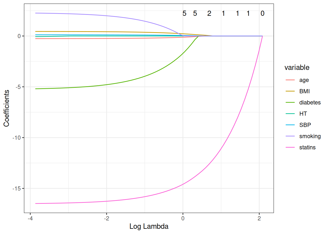
## Example: LASSO for LDL
::: {#fig-lasso-ldl}
```{r}
library(glmnet)
library(ggfortify)

hers_ldl_complete <-
  hers_ldl |>
  dplyr::select(LDL, HT, age, BMI, diabetes, smoking, statins, SBP) |>
  tidyr::drop_na()

y_ldl <- hers_ldl_complete$LDL
x_ldl <-
  hers_ldl_complete |>
  dplyr::select(-LDL) |>
  mutate(
    HT = as.integer(HT == "HT"),
    statins = as.integer(statins == "Yes"),
    diabetes = as.integer(diabetes == "Yes"),
    smoking = as.integer(smoking == "Yes")
  ) |>
  as.matrix()

lasso_fit <- glmnet(x_ldl, y_ldl)
autoplot(lasso_fit, xvar = "lambda") +
  theme_bw()
```
LASSO coefficient paths for LDL predictors in HERS.
Each line traces one predictor's coefficient as $\lambda$ increases.
Coefficients shrink toward zero as the penalty grows;
some reach exactly zero (variables excluded from the model).
:::
---
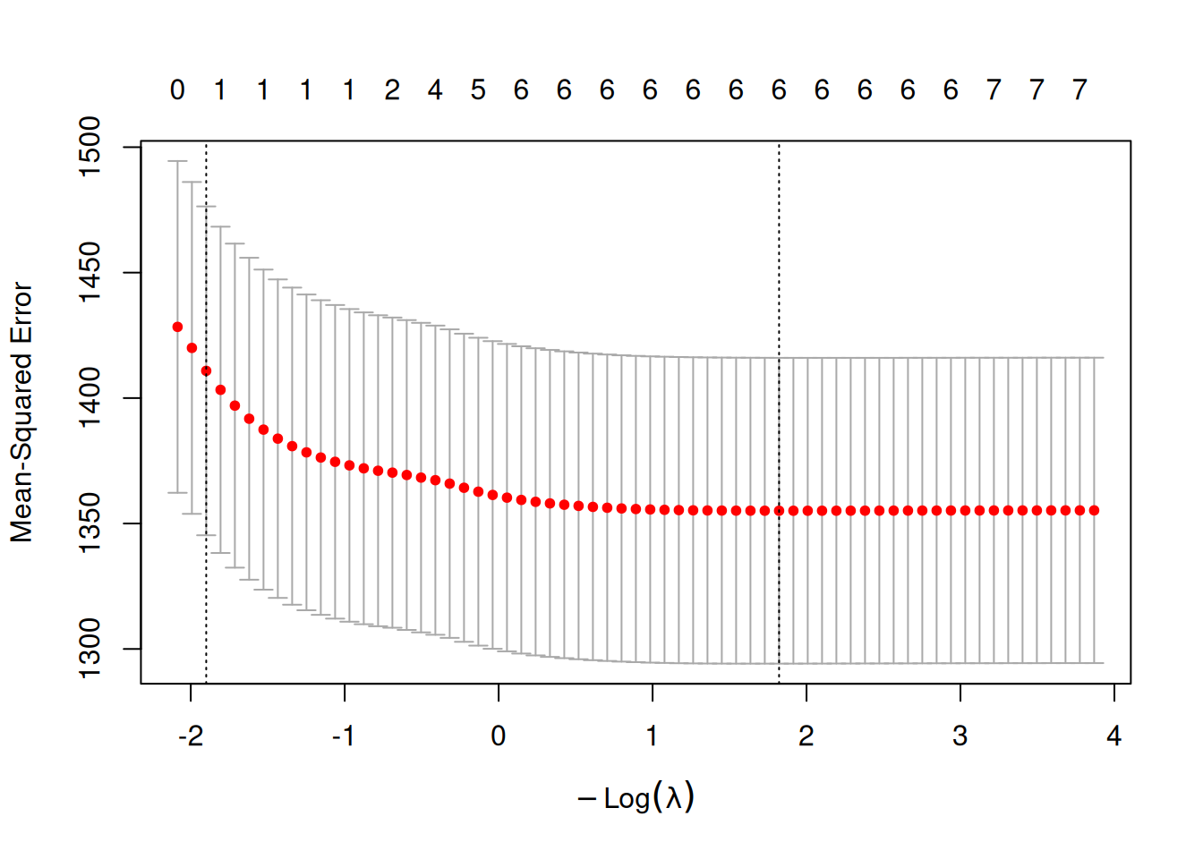
::: {#fig-lasso-cv}
```{r}
cv_lasso <- cv.glmnet(x_ldl, y_ldl)
plot(cv_lasso)
```
Cross-validated LASSO for LDL: mean squared error vs. $\log(\lambda)$.
The left dashed line marks `lambda.min` (minimum CV error);
the right dashed line marks `lambda.1se` (largest $\lambda$ within 1 SE of the minimum).
:::
---
::: {#tbl-lasso-coefs}
```{r}
data.frame(
  lambda.min = as.vector(coef(cv_lasso, s = "lambda.min")),
  lambda.1se = as.vector(coef(cv_lasso, s = "lambda.1se")),
  row.names = rownames(coef(cv_lasso))
)
```
LASSO coefficients at two values of the regularization parameter.
`lambda.min` minimizes cross-validation error;
`lambda.1se` uses a more conservative (larger) $\lambda$,
within one standard error of the minimum,
producing a sparser model.
:::
::: notes
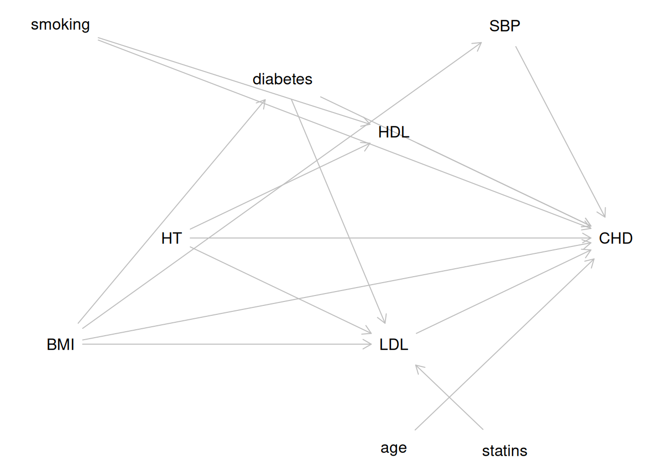
The LASSO identifies `statins` and `HT` as the strongest predictors
of LDL cholesterol in the HERS data,
consistent with the biological knowledge encoded in the DAG
in @fig-hers-dag.
:::
# Some Details {#sec-pred-sel-details}
{{< include _sec-pred-sel-details.qmd >}}
# Summary {#sec-pred-sel-summary}
Predictor selection is the process of choosing appropriate variables
for inclusion in a multivariable regression model.
The right approach depends on the **inferential goal**:
**For prediction** (Goal 1):
- Pre-specify well-motivated candidate predictors.
- Use cross-validation of a target PE measure
to select among models without overfitting.
- Shrinkage methods (LASSO, ridge) are effective
when there are many candidates.
**For evaluating a predictor of primary interest** (Goal 2):
- Use a DAG to identify confounders, mediators, and colliders.
- Include all well-established confounders for face validity.
- Use backward selection with a liberal criterion ($p < 0.2$)
to remove apparent non-confounders.
- In randomized trials, covariates are not required for confounding control
but improve precision (and de-attenuate estimates in logistic/Cox models).
- Pre-specify adjusted analyses in trial protocols.
**For identifying multiple important predictors** (Goal 3):
- Apply the same inclusive strategy as Goal 2.
- Consider the Allen–Cady modified backward selection procedure
to limit false-positive findings.
- Interpret novel, weak, and borderline significant associations
cautiously; report all candidate predictors considered.
**Across all goals**:
- Collinearity between a primary predictor and a confounder
can inflate standard errors; between adjustment variables, it does not.
- The EPV rule (10 events per predictor) flags potential problems
but is not a hard limit.
- Model selection complicates inference:
nominal p-values and confidence intervals are anticonservative
when predictors have been selected from the data.
# Learning Objectives {#sec-pred-sel-objectives .unnumbered}
After completing this chapter, students should be able to:
1. **Identify the inferential goal** of a predictor selection problem
(prediction, evaluating a primary predictor,
or identifying multiple important predictors)
and choose an appropriate strategy.
2. **Use a DAG** to identify confounders, mediators, and colliders,
and determine which covariates to include or exclude.
3. **Apply backward selection with a liberal criterion**
to select confounders in observational studies.
4. **Use AIC and BIC** to compare alternative models.
5. **Apply and interpret the LASSO**,
including cross-validated selection of $\lambda$.
6. **Explain why stepwise selection is problematic**
and describe its known pitfalls.
7. **Describe the bias–variance trade-off** and explain
why cross-validation provides a less optimistic estimate of PE
than naive within-sample measures.
8. **Identify and handle collinearity**,
including using the VIF and understanding its implications
for different inferential goals.
9. **Articulate how model selection complicates inference**
and describe best practices for reporting in each inferential context.
# References {.unnumbered}
::: {#refs}
:::