Data

---

Configuring R

Functions from these packages will be used throughout this document:

library(conflicted) # check for conflicting function definitions
# library(printr) # inserts help-file output into markdown output
library(rmarkdown) # Convert R Markdown documents into a variety of formats.
library(pander) # format tables for markdown
library(ggplot2) # graphics
library(ggfortify) # help with graphics
library(dplyr) # manipulate data
library(tibble) # `tibble`s extend `data.frame`s
library(magrittr) # `%>%` and other additional piping tools
library(haven) # import Stata files
library(knitr) # format R output for markdown
library(tidyr) # Tools to help to create tidy data
library(plotly) # interactive graphics
library(dobson) # datasets from Dobson and Barnett 2018
library(parameters) # format model output tables for markdown
library(haven) # import Stata files
library(latex2exp) # use LaTeX in R code (for figures and tables)
library(fs) # filesystem path manipulations
library(survival) # survival analysis
library(survminer) # survival analysis graphics
library(KMsurv) # datasets from Klein and Moeschberger
library(parameters) # format model output tables for
library(webshot2) # convert interactive content to static for pdf
library(forcats) # functions for categorical variables ("factors")
library(stringr) # functions for dealing with strings
library(lubridate) # functions for dealing with dates and times

Here are some R settings I use in this document:

rm(list = ls()) # delete any data that's already loaded into R

conflicts_prefer(dplyr::filter)
ggplot2::theme_set(
  ggplot2::theme_bw() + 
        # ggplot2::labs(col = "") +
    ggplot2::theme(
      legend.position = "bottom",
      text = ggplot2::element_text(size = 12, family = "serif")))

knitr::opts_chunk$set(message = FALSE)
options('digits' = 6)

panderOptions("big.mark", ",")
pander::panderOptions("table.emphasize.rownames", FALSE)
pander::panderOptions("table.split.table", Inf)
conflicts_prefer(dplyr::filter) # use the `filter()` function from dplyr() by default
legend_text_size = 9
run_graphs = TRUE

1 Types of variables

Before summarizing data, it helps to identify the type of each variable, since the appropriate descriptive methods depend on the type. Variables are broadly classified as either numerical or categorical, and within each class there are important subtypes.

---

Definition 1 (Numerical variable) A numerical (or quantitative) variable is a variable that takes values on a numeric scale, where arithmetic operations such as subtraction (and possibly division) are meaningful. Numerical variables may be further classified as interval or ratio variables, and as continuous or discrete.

Examples: age, blood pressure, cholesterol, number of cigarettes per day.

---

Definition 2 (Interval variable) An interval variable is a numerical variable for which differences between values are meaningful, but there is no natural zero point (so ratios of values are not meaningful).

Example: temperature in degrees Celsius — a difference of 10°C is meaningful, but 30°C is not “twice as hot” as 15°C.

---

Definition 3 (Ratio variable) A ratio variable is a numerical variable with a natural zero point, so that both differences and ratios of values are meaningful.

Examples: age, weight, cholesterol, blood pressure, number of cigarettes per day — a value of 0 means complete absence of the quantity.

---

Definition 4 (Continuous variable) A continuous variable is a numerical variable whose possible values form an interval (or union of intervals) of real numbers. A continuous variable is always numerical.

Examples: age, blood pressure, cholesterol, BMI.

---

Definition 5 (Discrete variable) A discrete variable is a variable whose possible values form a countable set. Discrete variables include both numerical types (such as count variables) and categorical types (such as binary, nominal, and ordinal variables). In contrast, continuous variables are always numerical.

Examples: number of cigarettes per day (discrete numerical/count), CHD event status (discrete categorical/binary).

---

Definition 6 (Categorical variable) A categorical (or qualitative) variable is a variable that takes values in a finite set of categories, where arithmetic operations such as differences are not meaningful. Categorical variables may be nominal (unordered) or ordinal (ordered), and are always discrete.

Examples: behavioral pattern (Type A1, A2, B3, B4), race/ethnicity, self-reported health status.

---

Definition 7 (Nominal variable) A nominal variable is a categorical variable whose categories have no natural ordering.

Examples: behavioral pattern (Type A1, A2, B3, B4), race/ethnicity, blood type.

---

Definition 8 (Ordinal variable) An ordinal variable is a categorical variable whose categories have a natural ordering.

Examples: self-reported health (poor, fair, good, very good, excellent), weight category.

---

Definition 9 (Binary variable) A binary variable takes only two possible values, often coded 0 (absence) and 1 (presence). A binary variable is a special case of a nominal variable.

Examples: CHD event (yes/no), current smoker (yes/no).

---

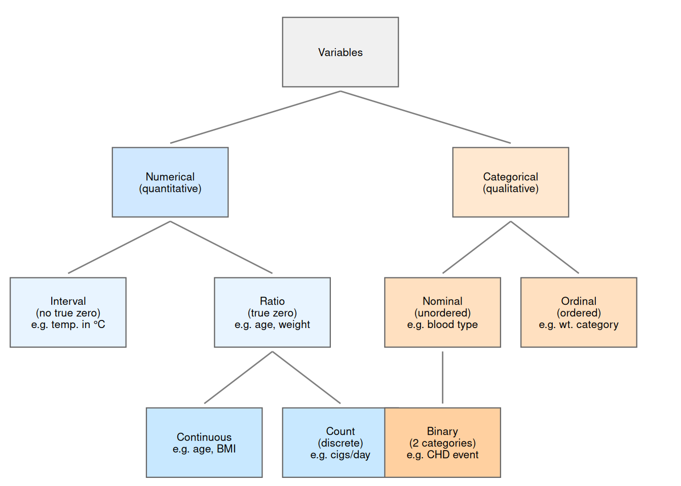
Figure 1 illustrates the relationships among these variable types.

nodes <- tibble::tribble(
  ~id,   ~x,    ~y,   ~label,
  "V",    5,    4.5,  "Variables",
  "N",    2.5,  3,    "Numerical\n(quantitative)",
  "C",    7.5,  3,    "Categorical\n(qualitative)",
  "I",    1,    1.5,  "Interval\n(no true zero)\ne.g. temp. in \u00b0C",
  "R",    4,    1.5,  "Ratio\n(true zero)\ne.g. age, weight",
  "CT",   3,    0,    "Continuous\ne.g. age, BMI",
  "CNT",  5,    0,    "Count\n(discrete)\ne.g. cigs/day",
  "NOM",  6.5,  1.5,  "Nominal\n(unordered)\ne.g. blood type",
  "ORD",  8.5,  1.5,  "Ordinal\n(ordered)\ne.g. wt. category",
  "BIN",  6.5,  0,    "Binary\n(2 categories)\ne.g. CHD event"
)
edges <- tibble::tribble(
  ~from, ~to,
  "V",   "N",
  "V",   "C",
  "N",   "I",
  "N",   "R",
  "R",   "CT",
  "R",   "CNT",
  "C",   "NOM",
  "C",   "ORD",
  "NOM", "BIN"
) |>
  dplyr::left_join(
    dplyr::select(nodes, id, x, y),
    by = c("from" = "id")
  ) |>
  dplyr::rename(x_from = x, y_from = y) |>
  dplyr::left_join(
    dplyr::select(nodes, id, x, y),
    by = c("to" = "id")
  ) |>
  dplyr::rename(x_to = x, y_to = y)
fill_colors <- c(
  "V" = "#f0f0f0",
  "N" = "#d0e8ff", "C" = "#ffe8d0",
  "I" = "#e8f4ff", "R" = "#e8f4ff",
  "CT" = "#c8e8ff", "CNT" = "#c8e8ff",
  "NOM" = "#ffe0c0", "ORD" = "#ffe0c0",
  "BIN" = "#ffd0a0"
)
ggplot2::ggplot() +
  ggplot2::aes() +
  ggplot2::geom_segment(
    data = edges,
    ggplot2::aes(
      x = x_from, y = y_from - 0.45,
      xend = x_to, yend = y_to + 0.45
    ),
    color = "grey50"
  ) +
  ggplot2::geom_tile(
    data = nodes,
    ggplot2::aes(x = x, y = y, fill = id),
    width = 1.7, height = 0.8,
    color = "grey40", linewidth = 0.4,
    show.legend = FALSE
  ) +
  ggplot2::geom_text(
    data = nodes,
    ggplot2::aes(x = x, y = y, label = label),
    size = 2.8, lineheight = 0.9
  ) +
  ggplot2::scale_fill_manual(values = fill_colors) +
  ggplot2::scale_y_continuous(
    limits = c(-0.5, 5.1), expand = c(0, 0)
  ) +
  ggplot2::scale_x_continuous(
    limits = c(0, 10), expand = c(0, 0)
  ) +
  ggplot2::theme_void()

Figure 1: Taxonomy of variable types. Count variables are discrete and numerical; binary, nominal, and ordinal variables are discrete and categorical.

Note

The continuous/discrete distinction cuts across the numerical/categorical distinction. Continuous variables are always numerical. Discrete variables include both numerical types (e.g., count variables) and categorical types (e.g., binary, nominal, and ordinal variables).

---

Table 1 shows selected variables from the WCGS dataset and their types.

tibble::tribble(
  ~Variable, ~Description, ~Type, ~Scale,
  "`age`", "Age (years)", "Continuous", "Ratio",
  "`chol`", "Total cholesterol", "Continuous", "Ratio",
  "`sbp`", "Systolic blood pressure", "Continuous", "Ratio",
  "`bmi`", "Body mass index (kg/m²)", "Continuous", "Ratio",
  "`weight`", "Weight (lbs)", "Continuous", "Ratio",
  "`ncigs`", "Cigarettes per day", "Count (discrete)", "Ratio",
  "`chd69`", "CHD event by 1969", "Binary (nominal)", "Nominal",
  "`smoke`", "Current smoking", "Binary (nominal)", "Nominal",
  "`arcus`", "Arcus senilis", "Binary (nominal)", "Nominal",
  "`dibpat`", "Behavioral pattern (A/B)", "Binary (nominal)", "Nominal",
  "`behpat`", "Behavioral pattern (A1/A2/B3/B4)", "Nominal", "Nominal",
  "`wghtcat`", "Weight category", "Ordinal", "Ordinal",
  "`agec`", "Age group", "Ordinal", "Ordinal"
) |>
  knitr::kable()

Table 1: Selected WCGS variables and their types

Variable	Description	Type	Scale
age	Age (years)	Continuous	Ratio
chol	Total cholesterol	Continuous	Ratio
sbp	Systolic blood pressure	Continuous	Ratio
bmi	Body mass index (kg/m²)	Continuous	Ratio
weight	Weight (lbs)	Continuous	Ratio
ncigs	Cigarettes per day	Count (discrete)	Ratio
chd69	CHD event by 1969	Binary (nominal)	Nominal
smoke	Current smoking	Binary (nominal)	Nominal
arcus	Arcus senilis	Binary (nominal)	Nominal
dibpat	Behavioral pattern (A/B)	Binary (nominal)	Nominal
behpat	Behavioral pattern (A1/A2/B3/B4)	Nominal	Nominal
wghtcat	Weight category	Ordinal	Ordinal
agec	Age group	Ordinal	Ordinal

2 Random variables

2.1 Binary variables

Definition 10 (binary variable) A binary variable is a random variable which has only two possible values in its range.

Exercise 1 (Examples of binary variables) What are some examples of binary variables in the health sciences?

---

NoteSolution

Solution. Examples of binary outcomes include:

• exposure (exposed vs unexposed)
• disease (diseased vs healthy)
• recovery (recovered vs unrecovered)
• relapse (relapse vs remission)
• return to hospital (returned vs not)
• vital status (dead vs alive)

---

2.2 Count variables

Definition 11 (Count variable) A count variable is a random variable whose possible values are some subset of the non-negative integers; that is, a random variable \(X\) such that:

\[\mathcal{R}(X) \in \text{N}\]

---

Exercise 2 What are some examples of count variables?

---

NoteSolution

Solution.

• Number of fish in a pond
• Number of cyclones per season
• Seconds of tooth-brushing per session (if rounded)
• Infections per person-year
• Visits to ER per person-month
• Car accidents per 1000 miles driven

---

Probability distributions for count outcomes

• Poisson distribution

• Negative binomial distribution

---