rm(list =ls())# delete any data that's already loaded into Rconflicts_prefer(dplyr::filter)ggplot2::theme_set(ggplot2::theme_bw()+# ggplot2::labs(col = "") +ggplot2::theme( legend.position ="bottom", text =ggplot2::element_text(size =12, family ="serif")))knitr::opts_chunk$set(message =FALSE)options('digits'=6)panderOptions("big.mark", ",")pander::panderOptions("table.emphasize.rownames", FALSE)pander::panderOptions("table.split.table", Inf)conflicts_prefer(dplyr::filter)# use the `filter()` function from dplyr() by defaultlegend_text_size=9run_graphs=TRUE
2 Welcome
Welcome to Epidemiology 204: Quantitative Epidemiology III (Statistical Models).
Epi 204 is a course on regression modeling.
3 What you should already know
Warning
Epi 202, Epi 203, and Sta 108 are prerequisites for this course. If you haven’t passed one of these courses, talk to me ASAP.
3.0.1 Epi 202: probability models
Probability distributions
binomial
Poisson
Gaussian
exponential
Characteristics of probability distributions
Mean, median, mode, quantiles
Variance, standard deviation, overdispersion
Characteristics of samples
independence, dependence, covariance, correlation
ranks, order statistics
identical vs nonidentical distribution (homogeneity vs heterogeneity)
Laws of Large Numbers
Central Limit Theorem for the mean of an iid sample
3.0.2 Epi 203: inference for one or several homogenous populations
the maximum likelihood inference framework:
likelihood functions
log-likelihood functions
score functions
estimating equations
information matrices
point estimates
standard errors
confidence intervals
hypothesis tests
p-values
Hypothesis tests for one, two, and >2 groups:
t-tests/ANOVA for Gaussian models
chi-square tests for binomial and Poisson models
nonparametric tests:
Wilcoxon signed-rank test for matched pairs
Mann–Whitney/Kruskal-Wallis rank sum test for \(\geq 2\) independent samples
Fisher’s exact test for contingency tables
Cochran–Mantel–Haenszel-Cox log-rank test
For all of the quantities above, and especially for confidence intervals and p-values, you should know how both:
Linear (Gaussian) regression models (review and more details)
Regression models for non-Gaussian outcomes
binary
count
time to event
Statistical analysis using R
We will start where Epi 203 left off: with linear regression models.
5 Motivations for regression models
Exercise 1 Why do we need regression models?
NoteSolution
Solution 1.
when there’s not enough data to analyze every subgroup of interest individually
especially when subgroups are defined using continuous predictors
5.1 Uses of regression models
Vittinghoff et al. (2012, sec. 1.3) identifies three broad motivations for using multipredictor regression models:
Multipredictor regression can be a powerful tool for addressing three important practical questions. … [These] include prediction, isolating the effect of a single predictor, and understanding multiple predictors.
Prediction: “Multipredictor regression is a powerful and general tool for using multiple measured predictors to make useful predictions for future observations.”
Isolating the Effect of a Single Predictor: “In settings where multiple, related predictors contribute to study outcomes, it will be important to consider multiple predictors even when a single predictor is of interest.” (e.g., to minimize confounding and support causal interpretation)
Understanding Multiple Predictors: “Multipredictor regression can also be used when our aim is to identify multiple independent predictors of a study outcome — independent in the sense that they appear to have an effect over and above other measured variables.” (including mediation and interaction)
Kleinbaum et al. (2014, sec. 4.1) provides a more granular list of eight overlapping applications of regression analysis:
In practice, a regression analysis is appropriate for several possibly overlapping situations, including the following:
Characterize the association: “You want to characterize the relationship between the dependent and independent variables by determining the extent, direction, and strength of the association.”
Prediction: “You seek a quantitative formula or equation to describe (e.g., predict) the dependent variable \(Y\) as a function of the independent variables \(X_1, X_2, \ldots, X_k\).”
Controlled description: “You want to describe quantitatively or qualitatively the relationship between \(X_1, X_2, \ldots, X_k\) and \(Y\) but control for the effects of still other variables \(X_{k+1}, X_{k+2}, \ldots, X_{k+p}\), which you believe have an important relationship with the dependent variable.”
Variable selection: “You want to determine which of several independent variables are important and which are not for describing or predicting a dependent variable. You may want to control for other variables. You may also want to rank independent variables in their order of importance.”
Model selection: “You want to determine the best mathematical model for describing the relationship between a dependent variable and one or more independent variables.”
Comparing regression relationships: “You want to compare several derived regression relationships.” (e.g., whether a relationship between two variables differs across subgroups)
Interaction: “You want to assess the interactive effects of two or more independent variables with regard to a dependent variable.”
Adjusted coefficient estimation: “You want to obtain a valid and precise estimate of one or more regression coefficients from a larger set of regression coefficients in a given model.” (i.e., estimating the effect of one variable after adjusting for others)
5.1.1 Relating the two lists
The two lists use different levels of granularity to describe the same landscape of regression uses. Vittinghoff et al. (2012) provides three broad categories, while Kleinbaum et al. (2014) identifies eight more specific applications.
Table 1: Comparing the categorizations of regression model uses in Vittinghoff et al. (2012, sec. 1.3) and Kleinbaum et al. (2014, sec. 4.1)
Vittinghoff et al. (2012)’s “Prediction” corresponds directly to Kleinbaum et al. (2014)’s Application 2.
Vittinghoff et al. (2012)’s “Isolating the Effect of a Single Predictor” corresponds to Kleinbaum et al. (2014)’s Application 8, which specifically targets accurate estimation of a single adjusted coefficient after controlling for other variables in the model.
Vittinghoff et al. (2012)’s “Understanding Multiple Predictors” is the broadest category, encompassing Applications 1, 3, 4, 5, 6, and 7: characterizing the overall association structure (Application 1), describing multiple predictors while controlling for confounders (Application 3), determining which variables matter (Application 4), finding the best-fitting model form (Application 5), comparing regression relationships across subgroups (Application 6), and assessing interaction effects (Application 7).
Applications 6 and 7 are related but distinct: Application 6 asks whether a derived regression relationship (e.g., a coefficient or the overall model) differs across pre-defined groups, typically by comparing models fit separately for each group. Application 7 asks whether two predictors interact within a single model — that is, whether the effect of one predictor on the outcome depends on the value of another predictor. In that sense, Application 6 can be viewed as a special case of Application 7 where the grouping variable is the effect modifier.
The key conceptual distinction made by Vittinghoff et al. (2012) — but not explicitly highlighted by Kleinbaum et al. (2014) — is between prediction (forecasting future outcomes) and causal inference (estimating the effect of a specific predictor). This distinction has important implications for model building strategy: prediction models can include any variables that improve predictive accuracy, while causal inference requires careful consideration of confounding, mediation, and the causal structure of the data.
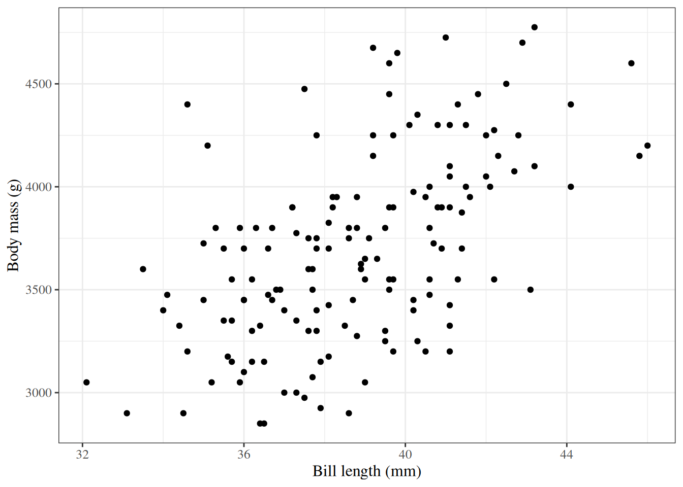
5.2 Example: Adelie penguins
Figure 1: Palmer penguins
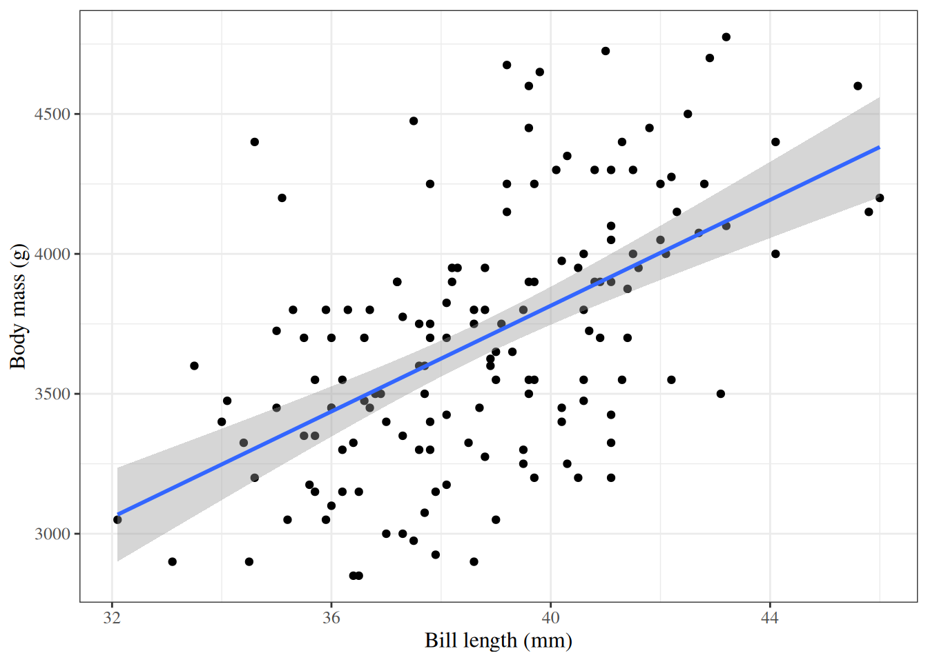
5.3 Linear regression
Show R code
ggpenguins2<-ggpenguins+stat_smooth( method ="lm", formula =y~x, geom ="smooth")ggpenguins2|>print()
Figure 2: Palmer penguins with linear regression fit
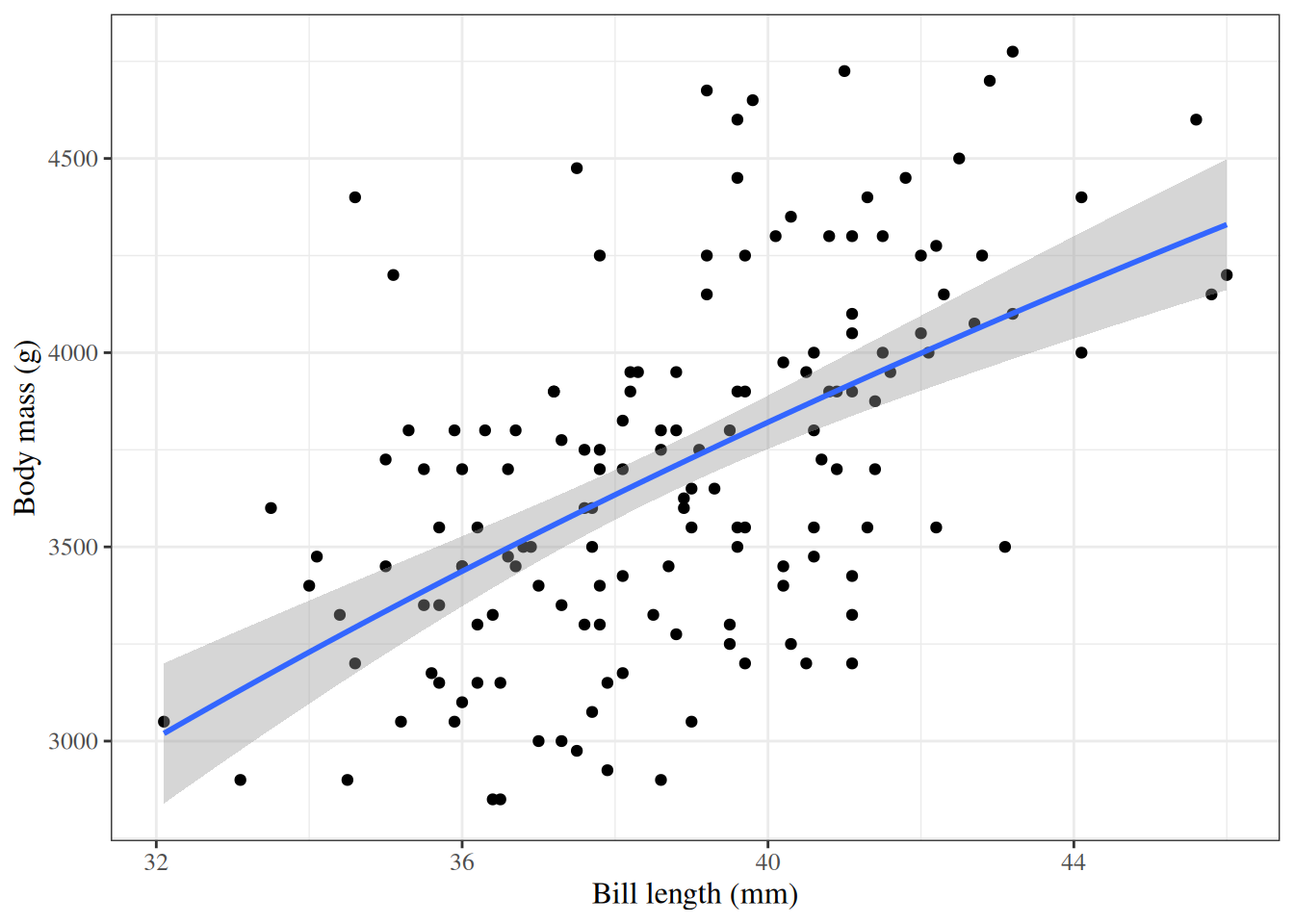
5.4 Curved regression lines
Show R code
ggpenguins2<-ggpenguins+stat_smooth( method ="lm", formula =y~log(x), geom ="smooth")+xlab("Bill length (mm)")+ylab("Body mass (g)")ggpenguins2
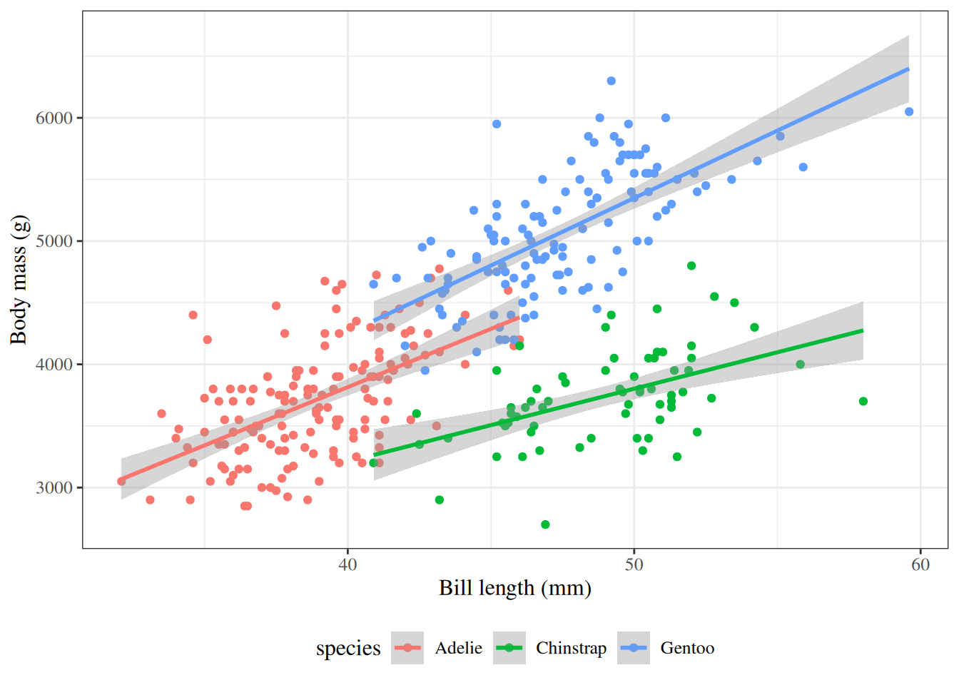
ggpenguins<-palmerpenguins::penguins|>ggplot(aes( x =bill_length_mm, y =body_mass_g, color =species))+geom_point()+stat_smooth( method ="lm", formula =y~x, geom ="smooth")+xlab("Bill length (mm)")+ylab("Body mass (g)")ggpenguins|>print()
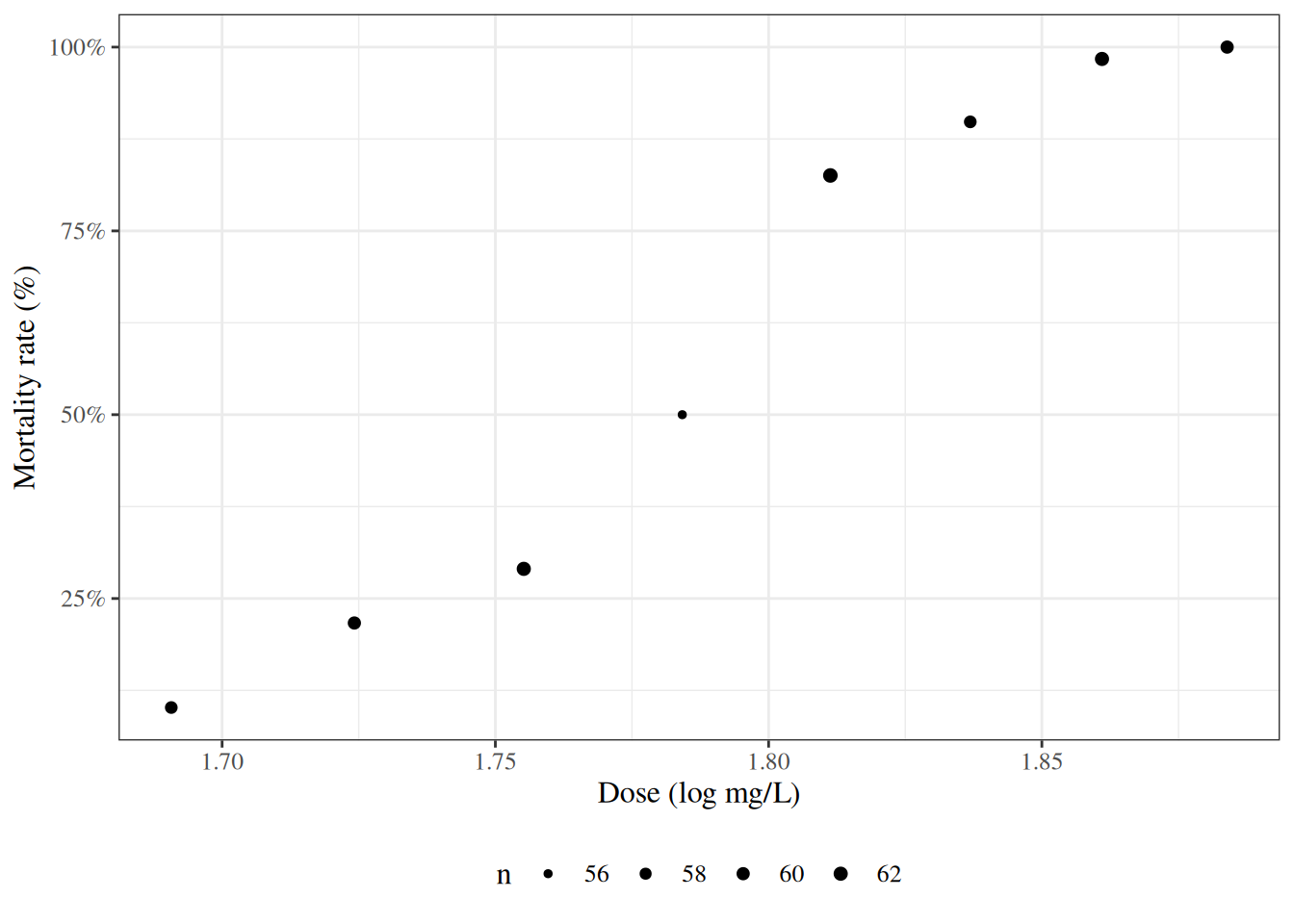
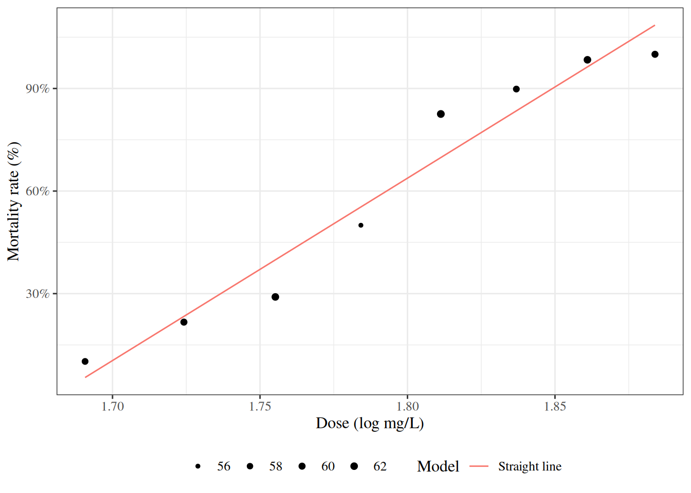
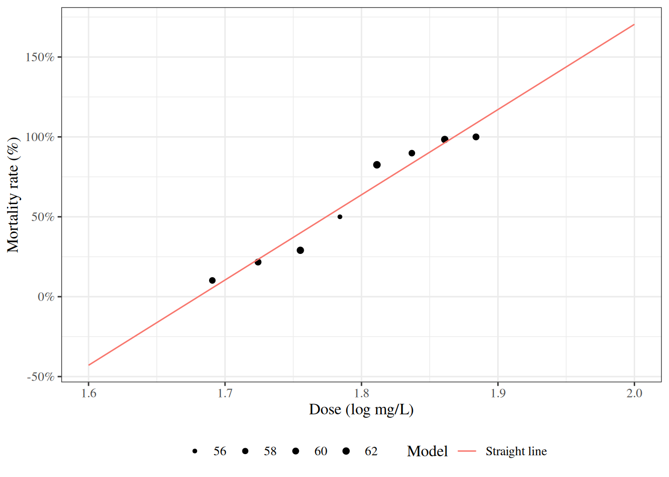
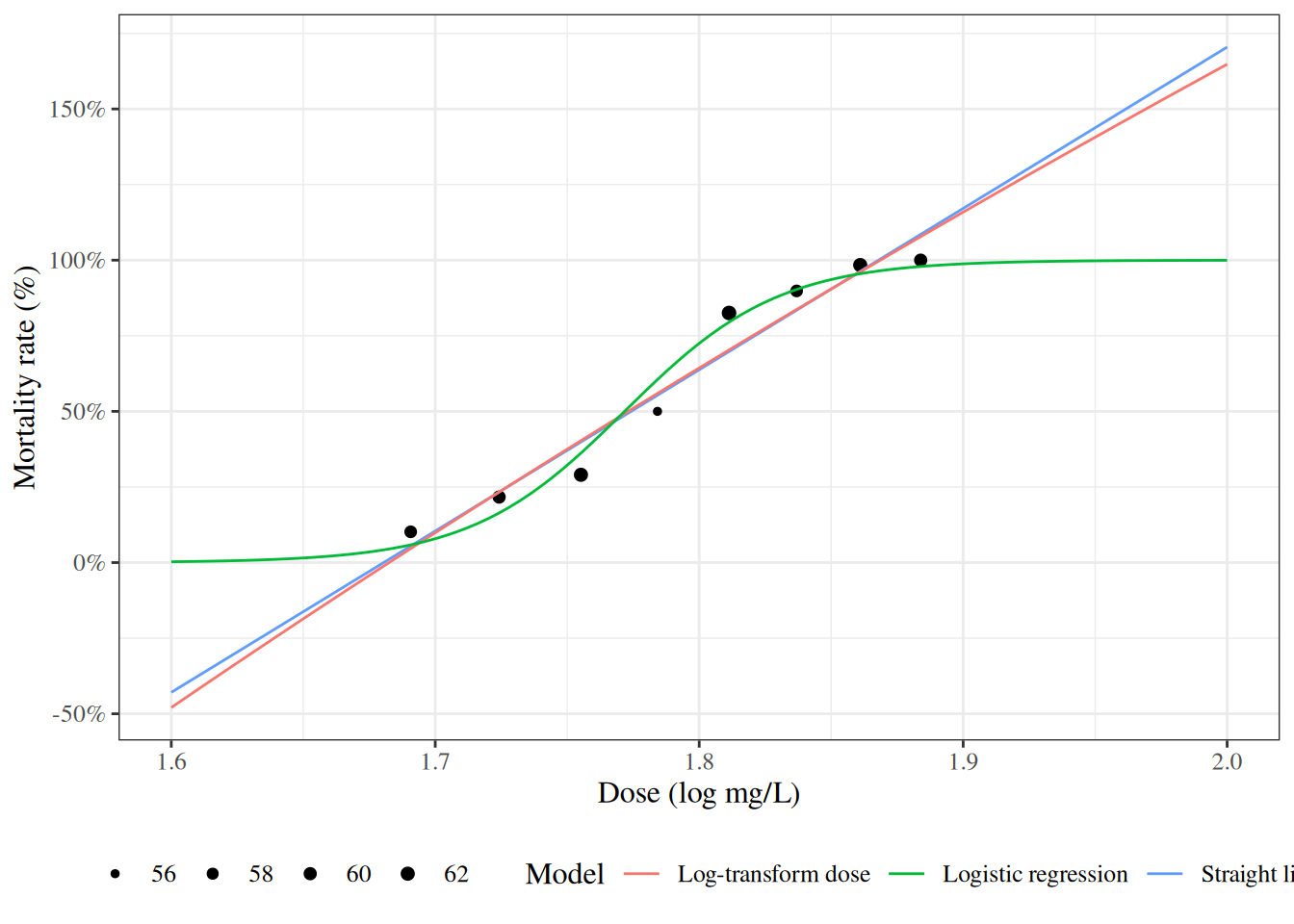
Figure 8: Mortality rates of adult flour beetles after five hours’ exposure to gaseous carbon disulphide (Bliss 1935)
5.10 Logistic regression
Show R code
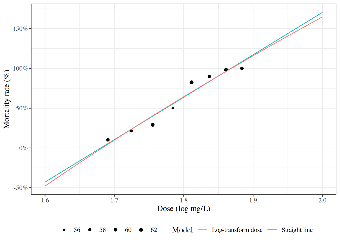
glm1<-beetles|>glm(formula =cbind(died, survived)~dose, family ="binomial")f<-function(x){glm1|>predict(newdata =data.frame(dose =x), type ="response")}plot4<-plot3+geom_function(fun =f, aes(col ="Logistic regression"))print(plot4)
Figure 9: Mortality rates of adult flour beetles after five hours’ exposure to gaseous carbon disulphide (Bliss 1935)
6 Structure of regression models
Exercise 2 What is a regression model?
Definition 1 (Regression model) Regression models are conditional probability distribution models:
\[\text{P}(Y|\tilde{X})\]
Exercise 3 What are some of the names used for the variables in a regression model \(\text{P}(Y|\tilde{X})\)?
Definition 2 (Outcome) The outcome variable in a regression model is the variable whose distribution is being described; in other words, the variable on the left-hand side of the “|” (“pipe”) symbol.
The outcome variable is also called the response variable, regressand, predicted variable, explained variable, experimental variable, output variable, dependent variable, endogenous variables, target, or label.
and is typically denoted \(Y\).
Definition 3 (Predictors) The predictor variables in a regression model are the conditioning variables defining subpopulations among which the outcome distribution might vary.
Predictors are also called regressors, covariates, independent variables, explanatory variables, risk factors, exposure variables, input variables, exogenous variables, candidate variables (Dunn and Smyth (2018)), carriers (Dunn and Smyth (2018)), manipulated variables, or features and are typically denoted \(\tilde{X}\). 1
Table 2: Common pairings of terms for variables \(\tilde{X}\) and \(Y\) in regression models \(P(Y|\tilde{X})\)2
\(\tilde{X}\)
\(Y\)
usual context
input
output
independent
dependent
predictor
predicted or response
explanatory
explained
exogenous
endogenous
econometrics
manipulated
measured
randomized controlled experiments
exposure
outcome
epidemiology
feature
label or target
machine learning
Exercise 4 What is the general structure of a generalized linear model?
NoteSolution
Solution 2. Generalized linear models have three components:
The outcome distribution family: \(\text{p}(Y|\mu(\tilde{x}))\)
The link function: \(g(\mu(\tilde{x})) = \eta(\tilde{x})\)
The linear component: \(\eta(\tilde{x}) = \tilde{x}\cdot \beta\)
The outcome distribution family (a.k.a. the random component of the model)
Gaussian (normal)
Binomial
Poisson
Exponential
Gamma
Negative binomial
The linear component (a.k.a. the linear predictor or linear functional form) describing how the covariates combine to define subpopulations:
Vittinghoff, Eric, David V Glidden, Stephen C Shiboski, and Charles E McCulloch. 2012. Regression Methods in Biostatistics: Linear, Logistic, Survival, and Repeated Measures Models. 2nd ed. Springer. https://doi.org/10.1007/978-1-4614-1353-0.
Wickham, Hadley, Mine Çetinkaya-Rundel, and Garrett Grolemund. 2023. R for Data Science. " O’Reilly Media, Inc.". https://r4ds.hadley.nz/.
The “~” (“tilde”) symbol in the notation \(\tilde{X}\) indicates that \(\tilde{X}\) is a vector. See the appendices for a table of notation used in these notes.↩︎