Measures of Association for Binary Outcomes

Risks, odds, odds ratios, and the logit and expit functions

---

Configuring R

Functions from these packages will be used throughout this document:

library(conflicted) # check for conflicting function definitions
# library(printr) # inserts help-file output into markdown output
library(rmarkdown) # Convert R Markdown documents into a variety of formats.
library(pander) # format tables for markdown
library(ggplot2) # graphics
library(ggfortify) # help with graphics
library(dplyr) # manipulate data
library(tibble) # `tibble`s extend `data.frame`s
library(magrittr) # `%>%` and other additional piping tools
library(haven) # import Stata files
library(knitr) # format R output for markdown
library(tidyr) # Tools to help to create tidy data
library(plotly) # interactive graphics
library(dobson) # datasets from Dobson and Barnett 2018
library(parameters) # format model output tables for markdown
library(haven) # import Stata files
library(latex2exp) # use LaTeX in R code (for figures and tables)
library(fs) # filesystem path manipulations
library(survival) # survival analysis
library(survminer) # survival analysis graphics
library(KMsurv) # datasets from Klein and Moeschberger
library(parameters) # format model output tables for
library(webshot2) # convert interactive content to static for pdf
library(forcats) # functions for categorical variables ("factors")
library(stringr) # functions for dealing with strings
library(lubridate) # functions for dealing with dates and times
library(broom) # Summarizes key information about statistical objects in tidy tibbles
library(broom.helpers) # Provides suite of functions to work with regression model 'broom::tidy()' tibbles

Here are some R settings I use in this document:

rm(list = ls()) # delete any data that's already loaded into R

conflicts_prefer(dplyr::filter)
ggplot2::theme_set(
  ggplot2::theme_bw() + 
        # ggplot2::labs(col = "") +
    ggplot2::theme(
      legend.position = "bottom",
      text = ggplot2::element_text(size = 12, family = "serif")))

knitr::opts_chunk$set(message = FALSE)
options('digits' = 6)

panderOptions("big.mark", ",")
pander::panderOptions("table.emphasize.rownames", FALSE)
pander::panderOptions("table.split.table", Inf)
conflicts_prefer(dplyr::filter) # use the `filter()` function from dplyr() by default
legend_text_size = 9
run_graphs = TRUE

options(digits = 6)

Acknowledgements

This content is adapted from:

• Dobson and Barnett (2018), Chapter 7
• Vittinghoff et al. (2012), Chapter 5
• David Rocke’s materials from the 2021 edition of Epi 204
• Nahhas (2024) Chapter 6

1 Introduction

This chapter reviews measures of association for binary outcomes: risks, risk differences, risk ratios, odds, and odds ratios, along with the logit and expit functions that connect probabilities, odds, and log-odds. These concepts are the vocabulary for regression models of binary outcomes; the logistic regression chapter builds on them.

1.1 Risk estimation and prediction

In Epi 203, you have already seen methods for modeling binary outcomes using one covariate that is also binary (such as exposure/non-exposure). In this section, we review one-covariate analyses, with a special focus on risk ratios and odds ratios, which are important concepts for interpreting logistic regression.

Exm

Example 1 (Oral Contraceptive Use and Heart Attack)  

• Research question: how does oral contraceptive (OC) use affect the risk of myocardial infarction (MI; a.k.a. heart attack)?

This was a concern when oral contraceptives were first developed, because the original formulations used much higher doses of estrogen than are used today. Cardiovascular risk from combined oral contraceptives increases with estrogen dose, and the dose has been reduced substantially since those early formulations, so modern low-dose formulations carry much lower risk (Roach et al. 2015).

Table 1 contains simulated data for an imaginary follow-up (a.k.a. prospective) study in which two groups are identified, one using OCs and another not using OCs, and both groups are tracked for three years to determine how many in each groups have MIs.

library(dplyr)
oc_mi <-
  tribble(
    ~OC, ~MI, ~Total,
    "OC use", 13, 5000,
    "No OC use", 7, 10000
  ) |>
  mutate(`No MI` = Total - MI) |>
  relocate(`No MI`, .after = MI)

totals <-
  oc_mi |>
  summarize(across(c(MI, `No MI`, Total), sum)) |>
  mutate(OC = "Total")

tbl_oc_mi <- bind_rows(oc_mi, totals)

tbl_oc_mi |> pander::pander()

Table 1: Simulated data from study of oral contraceptive use and heart attack risk

OC	MI	No MI	Total
OC use	13	4,987	5,000
No OC use	7	9,993	10,000
Total	20	14,980	15,000

Exercise 1 Estimate the probabilities of MI for OC users and non-OC users in Example 1.

SolutionSolution

Solution 1. \[\mathop{\hat{\operatorname{p}}}\nolimits(MI|OC) = \frac{13}{5000} = 0.0026\]

\[\mathop{\hat{\operatorname{p}}}\nolimits(MI|\neg OC) = \frac{7}{10000} = 7\times 10^{-4}\]

Exercise 2 What does the term “controls” mean in the context of study design?

SolutionSolution

Solution 2.

Definition 1 (Two meanings of “controls”) Depending on context, “controls” can mean either:

• individuals who don’t experience an exposure of interest,
• or individuals who don’t experience an outcome of interest.

Exercise 3 What types of studies do the two definitions of controls correspond to?

SolutionSolution

Solution 3.

Definition 2 (cases and controls in retrospective studies) In retrospective case-control studies, participants who experience the outcome of interest are called cases, while participants who don’t experience that outcome are called controls (Rothman et al. 2021, chap. 8).

Definition 3 (treatment groups and control groups in prospective studies) In prospective studies, the group of participants who experience the treatment or exposure of interest is called the treatment group, while the participants who receive the baseline or comparison treatment (for example, clinical trial participants who receive a placebo or a standard-of-care treatment rather than an experimental treatment) are called controls (Rothman et al. 2021, chap. 7).

Exm

Example 2 (Cases and controls in the OC-MI study) Example 1 describes a prospective (follow-up) study: participants were enrolled based on their exposure status (OC use versus no OC use) and then followed for three years to observe MI outcomes.

Therefore, Definition 3 applies: the 5000 OC users form the treatment (exposed) group, and the 10,000 OC non-users are the controls.

Definition 2 does not apply to this study design, because participants were not selected based on their outcomes. If we had instead recruited participants by outcome status — enrolling the 20 participants who experienced MIs, along with a sample of participants who did not — the study would have been a retrospective case-control study: the 20 participants with MIs would be the cases, and the sampled MI-free participants would be the controls.

1.2 Comparing probabilities

1.2.1 Risk differences

The simplest comparison of two probabilities, \(\pi_1\), and \(\pi_2\), is the difference of their values:

Definition 4 (Risk difference) The risk difference of two probabilities, \(\pi_1\), and \(\pi_2\), is the difference of their values: \[\delta(\pi_1,\pi_2) \stackrel{\text{def}}{=}\pi_1 - \pi_2\]

Exm

Example 3 (Difference in MI risk) Here, we introduce the shorthand notation

\[\pi(OC) \stackrel{\text{def}}{=}\Pr(MI|OC), \quad \pi(\neg OC) \stackrel{\text{def}}{=}\Pr(MI|\neg OC)\]

for the probability of MI given OC use and given OC non-use, respectively.

In Example 1, the maximum likelihood estimate of the difference in MI risk between OC users and OC non-users is:

\[ \begin{aligned} \hat\delta(\pi(OC), \pi(\neg OC)) &= \delta(\hat\pi(OC), \hat\pi(\neg OC))\\ &= \hat\pi(OC) - \hat\pi(\neg OC)\\ &= 0.0026 - 7\times 10^{-4}\\ &= 0.0019 \end{aligned} \]

Exercise 4 (interpreting risk differences) How can we interpret the preceding risk difference estimate in prose?

SolutionSolution (interpreting risk differences)

Solution 4 (interpreting risk differences). “The difference in risk of MI between OC users and non-users was 0.0019.”

or

“The difference in risk of MI between OC users and non-users was 0.19 percentage points.”

See the note about working with percentages in the Appendix.

1.2.2 Risk ratios

Exercise 5 If \(\pi_1\) and \(\pi_2\) are two probabilities, what do we call the following ratio?

\[\rho(\pi_1,\pi_2) = \frac{\pi_1}{\pi_2}\]

SolutionSolution

Solution 5.

Definition 5 (Relative risk ratios) The ratio of two probabilities \(\pi_1\) and \(\pi_2\),

\[\rho(\pi_1,\pi_2) = \frac{\pi_1}{\pi_2}\]

is called the:

• risk ratio,
• relative risk ratio,
• probability ratio,
• or rate ratio

of \(\pi_1\) compared to \(\pi_2\).

Exercise 6  

In Solution 1, we estimated that:

\[\mathop{\hat{\operatorname{p}}}\nolimits(MI|OC) = 0.0026\]

\[\mathop{\hat{\operatorname{p}}}\nolimits(MI|\neg OC) = 7\times 10^{-4}\]

Now, estimate the relative risk of MI for OC versus non-OC.

SolutionSolution

Solution 6.

The relative risk of MI for OC versus non-OC is:

rr <- (13 / 5000) / (7 / 10000)

\[ \begin{aligned} \hat\rho(OC, \neg OC) &=\frac{\mathop{\hat{\operatorname{p}}}\nolimits(MI|OC)}{\mathop{\hat{\operatorname{p}}}\nolimits(MI|\neg OC)}\\ &= \frac{0.0026}{7\times 10^{-4}}\\ &= 3.714286 \end{aligned} \]

Exercise 7 How can we interpret the preceding relative risk estimate in prose?

SolutionSolution

Solution 7.

We might summarize this result by saying that:

• “The estimated probability of MI among OC users was 3.714286 times as high as the estimated probability among OC non-users.”

or

• “The estimated probability of MI among OC users was 2.714286 times higher than, the estimated probability among OC non-users.”

see also Vittinghoff et al. (2012, sec. 8.1.4), which uses similar phrasing.

1.2.3 Relative risk differences

The second approach in Solution 7, where we subtract 1 from the risk ratio, is actually reporting a slightly different metric:

Definition 6 (Relative risk difference)  

Sometimes, we divide the risk difference by the comparison probability; the result is called the relative risk difference:

\[\xi(\pi_1,\pi_2) \stackrel{\text{def}}{=}\frac{\delta(\pi_1,\pi_2)}{\pi_2}\]

Theorem 1 (Relative risk difference equals risk ratio minus 1) \[\xi(\pi_1,\pi_2) = \rho(\pi_1,\pi_2) - 1\]

ProofProof

Proof. \[ \begin{aligned} \xi(\pi_1,\pi_2) &\stackrel{\text{def}}{=}\frac{\delta(\pi_1,\pi_2)}{\pi_2} \\&= \frac{\pi_1-\pi_2}{\pi_2} \\&= \frac{\pi_1}{\pi_2} - 1 \\&= \rho(\pi_1,\pi_2) - 1 \end{aligned} \]

Exm

Example 4 (Relative difference in MI risk) In Example 1, the maximum likelihood estimate of the relative risk difference in MI risk between OC users and OC non-users is:

\[ \begin{aligned} \hat\xi(\pi(OC), \pi(\neg OC)) &= \xi(\hat\pi(OC), \hat\pi(\neg OC)) && \text{(invariance property of MLEs)} \\ &\stackrel{\text{def}}{=}\frac{\delta(\hat\pi(OC), \hat\pi(\neg OC))}{\hat\pi(\neg OC)} && \text{(definition of relative risk difference)} \\ &= \frac{0.0019}{7\times 10^{-4}} && \text{(substituting the estimates)} \\ &= 2.714286 && \text{(dividing)} \end{aligned} \]

The numerator 0.0019 is the risk difference estimate from Example 3, and the denominator 7^{-4} is the estimate \(\hat\pi(\neg OC)\) from Solution 1.

We can check this estimate using Theorem 1 and the risk ratio estimate from Solution 6:

\[ \begin{aligned} \hat\xi(\pi(OC), \pi(\neg OC)) &= \hat\rho(OC, \neg OC) - 1 && \text{(relative risk difference as risk ratio minus 1)} \\ &= 3.714286 - 1 && \text{(substituting the risk ratio estimate)} \\ &= 2.714286 && \text{(subtracting)} \end{aligned} \]

The two calculations agree.

1.2.4 Changing reference groups in risk comparisons

Risk differences, risk ratios, and relative risk differences are defined by two probabilities, plus a choice of which probability is the baseline or reference probability (i.e., which probability is the subtrahend of the risk difference or the denominator of the risk ratio).

\[\delta(\pi_2,\pi_1) = -\delta(\pi_1, \pi_2) \tag{1}\]

\[\rho(\pi_2,\pi_1) = \mathopen{}\left(\rho(\pi_1,\pi_2)\right)^{-1}\mathclose{} \tag{2}\]

\[\xi(\pi_2,\pi_1) = \mathopen{}\left(\xi(\pi_1,\pi_2) + 1\right)^{-1}\mathclose{} - 1 \tag{3}\]

Exercise 8 Prove Equation 1, Equation 2, and Equation 3.

SolutionSolution

Solution 8. To prove Equation 1:

\[ \begin{aligned} \delta(\pi_2,\pi_1) &\stackrel{\text{def}}{=}\pi_2 - \pi_1 && \text{(definition of risk difference)} \\ &= -(\pi_1 - \pi_2) && \text{(factoring out } -1 \text{)} \\ &= -\delta(\pi_1, \pi_2) && \text{(definition of risk difference)} \end{aligned} \]

To prove Equation 2:

\[ \begin{aligned} \rho(\pi_2,\pi_1) &\stackrel{\text{def}}{=}\frac{\pi_2}{\pi_1} && \text{(definition of risk ratio)} \\ &= \mathopen{}\left(\frac{\pi_1}{\pi_2}\right)^{-1}\mathclose{} && \text{(inverse of the inverted fraction)} \\ &= \mathopen{}\left(\rho(\pi_1,\pi_2)\right)^{-1}\mathclose{} && \text{(definition of risk ratio)} \end{aligned} \]

To prove Equation 3, first rearrange Theorem 1 to express the risk ratio in terms of the relative risk difference:

\[ \begin{aligned} \xi(\pi_1,\pi_2) &= \rho(\pi_1,\pi_2) - 1 && \text{(relative risk difference as risk ratio minus 1)} \\ \xi(\pi_1,\pi_2) + 1 &= \rho(\pi_1,\pi_2) && \text{(adding 1 to both sides)} \end{aligned} \]

Then apply Theorem 1 to the switched-reference pair \((\pi_2, \pi_1)\), substitute Equation 2, and substitute the rearranged form of Theorem 1:

\[ \begin{aligned} \xi(\pi_2,\pi_1) &= \rho(\pi_2,\pi_1) - 1 && \text{(relative risk difference as risk ratio minus 1)} \\ &= \mathopen{}\left(\rho(\pi_1,\pi_2)\right)^{-1}\mathclose{} - 1 && \text{(risk ratio with switched reference group)} \\ &= \mathopen{}\left(\xi(\pi_1,\pi_2) + 1\right)^{-1}\mathclose{} - 1 && \text{(substituting } \rho(\pi_1,\pi_2) = \xi(\pi_1,\pi_2) + 1 \text{)} \end{aligned} \]

Exm

Example 5 (Switching the reference group in a risk difference) In Example 3, we estimated that the risk difference of MI for OC versus non-OC is:

\[ \begin{aligned} \delta(OC, \neg OC) &= 0.0019 \end{aligned} \]

In comparison, the risk difference for non-OC versus OC is:

\[ \begin{aligned} \delta(\neg OC, OC) &= \mathop{\hat{\operatorname{p}}}\nolimits(MI|\neg OC) - \mathop{\hat{\operatorname{p}}}\nolimits(MI|OC)\\ &= 7\times 10^{-4} - 0.0026\\ &= -0.0019\\ &= -\delta(OC, \neg OC) \end{aligned} \]

as Equation 1 states.

Exm

Example 6 (Switching the reference group in a risk ratio) In Solution 6, we estimated that the risk ratio of OC versus non-OC is:

\[ \begin{aligned} \rho(OC, \neg OC) &= 3.714286 \end{aligned} \]

In comparison, the risk ratio for non-OC versus OC is:

\[ \begin{aligned} \rho(\neg OC, OC) &=\frac{\mathop{\hat{\operatorname{p}}}\nolimits(MI|\neg OC)}{\mathop{\hat{\operatorname{p}}}\nolimits(MI|OC)}\\ &= \frac{7\times 10^{-4}}{0.0026}\\ &= 0.269231\\ &= \frac{1}{\rho(OC, \neg OC)} \end{aligned} \]

as Equation 2 states.

Exm

Example 7 (Switching the reference group in a relative risk difference) In Example 4, we estimated that the relative risk difference of MI for OC versus non-OC is:

\[ \begin{aligned} \xi(OC, \neg OC) &= 2.714286 \end{aligned} \]

In comparison, the relative risk difference for non-OC versus OC is:

\[ \begin{aligned} \xi(\neg OC, OC) &= \frac{\mathop{\hat{\operatorname{p}}}\nolimits(MI|\neg OC) - \mathop{\hat{\operatorname{p}}}\nolimits(MI|OC)}{\mathop{\hat{\operatorname{p}}}\nolimits(MI|OC)}\\ &= \frac{-0.0019}{0.0026}\\ &= -0.730769 \end{aligned} \]

We can check this value against the switched-reference identity Equation 3:

\[ \begin{aligned} \frac{1}{\xi(OC, \neg OC) + 1} - 1 &= \frac{1}{2.714286 + 1} - 1\\ &= -0.730769 \end{aligned} \]

The two calculations agree.

1.3 Odds and odds ratios

1.3.1 Odds and probabilities

In logistic regression, we will make use of a mathematically-convenient transformation of probability, called odds:

Definition 7 (Odds)  

The odds of an event \(A\), is the probability that the event occurs, divided by the probability that it doesn’t occur. We can represent odds with the Greek letter \(\omega\) (“omega”). ¹ Thus, in mathematical notation:

\[\omega\stackrel{\text{def}}{=}\frac{\Pr(A)}{\Pr(\neg A)} \tag{4}\]

This course is about regression models, which are conditional probability models (regression models). Accordingly, we define conditional odds in terms of conditional probabilities:

Definition 8 (Conditional odds)  

The conditional odds of an event \(A\) given a condition \(B\), is the (conditional) probability that event \(A\) occurs (given condition \(B\)), divided by the (conditional) probability that it doesn’t occur (given condition \(B\)). In mathematical notation:

\[\omega(A|B) \stackrel{\text{def}}{=}\frac{\Pr(A|B)}{\Pr(\neg A|B)} \tag{5}\]

When the event \(A\) is clear from context, we abbreviate \(\omega(A|B)\) as \(\omega(B)\) or \(\omega_B\) (“omega bee”).

Definition 9 (Shorthand for MI risk under OC use) Let \(\pi(OC)\) denote the probability of MI given OC use:

\[\pi(OC) \stackrel{\text{def}}{=}\Pr(MI|OC)\]

Exm

Example 8 (Computing odds from probabilities) In Exercise 1, we estimated that \(\pi(OC) = 0.0026\) (Definition 9). If this estimate is correct, then the odds of MI, given OC use, is:

\[ \begin{aligned} \omega(OC) &\stackrel{\text{def}}{=}\frac{\Pr(MI|OC)}{\Pr(\neg MI|OC)}\\ &=\frac{\Pr(MI|OC)}{1-\Pr(MI|OC)}\\ &=\frac{\pi(OC)}{1-\pi(OC)}\\ &=\frac{0.0026}{1-0.0026}\\ &\approx 0.002607 \end{aligned} \]

Exercise 9 (Computing odds from probabilities) Estimate the odds of MI, for non-OC users.

SolutionSolution

Solution 9. \[ \omega(\neg OC) = 7.004903\times 10^{-4} \]

Exercise 10 Find a general formula for converting probabilities into odds.

SolutionSolution

Solution 10. Using Definition 7 and the complementary probability:

\[ \begin{aligned} \omega&\stackrel{\text{def}}{=}\frac{\Pr(A)}{\Pr(\neg A)} \\ &= \frac{\pi}{1-\pi} \end{aligned} \]

Theorem 2 (Odds as a function of probability) If \(\pi\) is the probability of an event \(A\) and \(\omega\) is the corresponding odds of \(A\), then:

\[\omega= \frac{\pi}{1-\pi} \tag{6}\]

ProofProof

Proof. By Solution 10.

The mathematical relationship between odds \(\omega\) and probabilities \(\pi\), which is represented in Equation 6, is a core component of logistic regression models, as we will see in the rest of this chapter. Let’s give the expression on the righthand side of Equation 6 its own name and symbol, so that we can refer to it concisely:

Definition 10 (Odds function) The odds function is defined as: \[\operatorname{odds}\mathopen{}\left\{\pi\right\}\mathclose{} \stackrel{\text{def}}{=}\frac{\pi}{1-\pi} \tag{7}\]

We can use the odds function (Definition 10) to simplify Equation 6 (in Theorem 2) into a more concise expression, which is easier to remember and manipulate:

Corollary 1 (Odds via the odds function) If \(\pi\) is the probability of an outcome \(A\) and \(\omega\) is the corresponding odds of \(A\), then:

\[\omega= \operatorname{odds}\mathopen{}\left\{\pi\right\}\mathclose{} \tag{8}\]

In other words, the odds function rescales probabilities into odds.

ProofProof

Proof. By Theorem 2 and Definition 10.

Exercise 11 Graph the odds function.

SolutionSolution

Solution 11.

Figure 1 graphs the odds function.

odds <- function(pi) pi / (1 - pi)
library(ggplot2)
ggplot() +
  geom_function(
    fun = odds,
    arrow = arrow(ends = "last"),
    mapping = aes(col = "odds function")
  ) +
  xlim(0, .99) +
  xlab("Probability") +
  ylab("Odds") +
  geom_abline(aes(
    intercept = 0,
    slope = 1,
    col = "y=x"
  )) +
  theme_bw() +
  labs(colour = "") +
  theme(legend.position = "bottom")

Figure 1: Odds versus probability

Theorem 3 (One-sample MLE for odds) Let \(X_1,...X_n\) be a set of \(n\) \(\operatorname{iid}\) Bernoulli trials, and let \(X = \sum_{i=1}^nX_i\) be their sum.

Then the maximum likelihood estimate of the common per-trial success odds \(\omega\) (that is, the odds of \(X_i=1\)) is:

\[ \hat{\omega}= \frac{x}{n-x} \]

ProofProof

Proof. \[ \begin{aligned} 1-\hat\pi &= 1-\frac{x}{n}\\ &= \frac{n}{n} - \frac{x}{n}\\ &= \frac{n - x}{n} \end{aligned} \]

Thus, the estimated odds is:

\[ \begin{aligned} \frac{\hat\pi}{1-\hat\pi} &= \frac{\left(\frac{x}{n}\right)}{\left(\frac{n-x}{n}\right)}\\ &= \frac{x}{n-x} \end{aligned} \tag{9}\]

That is, the odds estimate can be computed directly as “# events” divided by “# nonevents”, without needing to compute \(\hat\pi\) and \(1-\hat\pi\) first.

Exm

Example 9 (Calculating odds using the shortcut) In Example 8, we calculated \[ \begin{aligned} \omega(OC) &=0.002607 \end{aligned} \]

Let’s recalculate this result using our shortcut.

SolutionSolution

Solution 12. \[ \begin{aligned} \omega(OC) &=\frac{13}{5000-13}\\ &=0.002607 \end{aligned} \]

Same answer as in Example 8!

Theorem 4 (Simplified expressions for odds function)  

Two equivalent expressions for the odds function are:

\[ \begin{aligned} \operatorname{odds}\mathopen{}\left\{\pi\right\}\mathclose{} &= \frac{1}{\pi^{-1}-1} \\ &= \mathopen{}\left(\pi^{-1}-1\right)^{-1}\mathclose{} \end{aligned} \tag{10}\]

Exercise 12 Prove Theorem 4.

SolutionSolution

Solution 13. Starting from Definition 10:

\[ \begin{aligned} \operatorname{odds}\mathopen{}\left\{\pi\right\}\mathclose{} &= \frac{\pi}{1-\pi} \\ &= \frac{\pi}{1-\pi}\frac{\pi^{-1}}{\pi^{-1}} \\ &= \frac{\pi\pi^{-1}}{(1-\pi)\pi^{-1}} \\ &= \frac{1}{(\pi^{-1}-\pi\pi^{-1})} \\ &= \frac{1}{(\pi^{-1}-1)} \\ &= \mathopen{}\left(\pi^{-1}-1\right)^{-1}\mathclose{} \end{aligned} \]

Corollary 2 (Odds of a non-event) If \(\pi\) is the probability of event \(A\) and \(\omega\) is the corresponding odds of \(A\), then the odds of \(\neg A\) are:

\[ \begin{aligned} \omega(\neg A) &= \frac{1-\pi}{\pi} \\&= \pi^{-1}-1 \end{aligned} \]

ProofProof

Proof. Using Definition 7 (applied to the event \(\neg A\)) and the complement rule:

\[ \begin{aligned} \omega(\neg A) &\stackrel{\text{def}}{=}\frac{\Pr(\neg A)}{\Pr(\neg \neg A)} && \text{(definition of odds, applied to } \neg A\text{)} \\ &= \frac{\Pr(\neg A)}{\Pr(A)} && \text{(double negation: } \neg \neg A = A\text{)} \\ &= \frac{1-\pi}{\Pr(A)} && \text{(complement rule: } \Pr(\neg A) = 1-\pi\text{)} \\ &= \frac{1-\pi}{\pi} && \text{(} \Pr(A) = \pi \text{ by hypothesis)} \\ &= \frac{1}{\pi} - \frac{\pi}{\pi} && \text{(split the fraction)} \\ &= \frac{1}{\pi} - 1 && \text{(cancel: } \pi/\pi = 1\text{)} \\ &= \pi^{-1} - 1 && \text{(rewrite the reciprocal as a } -1 \text{ power)} \end{aligned} \]

Odds of rare events

Exercise 13 What odds value corresponds to the probability \(\pi = 0.2\), and what is the numerical difference between these two values?

SolutionSolution

Solution 14. The odds value corresponding to \(\pi = 0.2\) is:

\[ \omega= \frac{\pi}{1-\pi} =\frac{.2}{.8} = .25 \]

The numerical difference between the odds and the probability is:

\[ \omega- \pi = .25 - .2 = .05 \]

Exercise 14 Find the difference between an odds \(\omega\) and its corresponding probability \(\pi\), as a function of \(\pi\).

SolutionSolution

Solution 15. \[ \begin{aligned} \omega- \pi &= \frac{\pi}{1-\pi} - \pi \\ &= \frac{\pi}{1-\pi} - \frac{\pi(1-\pi)}{1-\pi} \\ &= \frac{\pi}{1-\pi} - \frac{\pi - \pi^2}{1-\pi} \\ &= \frac{\pi - (\pi - \pi^2)}{1-\pi} \\ &= \frac{\pi - \pi + \pi^2}{1-\pi} \\ &= \frac{\pi^2}{1-\pi} \\ &= \frac{\pi}{1-\pi} \pi \\ &= \omega\pi \end{aligned} \]

Theorem 5 (Difference between odds and probability) Let \(\omega= \frac{\pi}{1-\pi}\). Then:

\[\omega- \pi = \frac{\pi^2}{1-\pi}\]

ProofProof

Proof. By Solution 15.

For rare events (small \(\pi\)), odds and probabilities are nearly equal (see Figure 1), because \(1-\pi \approx 1\) and \(\pi^2 \approx 0\).

For example, in Example 8, the probability and odds differ by \(6.777622\times 10^{-6}\).

1.3.2 The inverse odds function

Exercise 15 If \(\pi\) is the probability of an event \(A\) and \(\omega\) is the corresponding odds of \(A\), how can we compute \(\pi\) from \(\omega\)?

For example, if \(\omega= 3/2\), what is \(\pi\)?

SolutionSolution

Solution 16. Starting from Theorem 2, we can solve Equation 6 for \(\pi\) in terms of \(\omega\):

\[ \begin{aligned} \omega&= \frac{\pi}{1-\pi} \\ (1-\pi) \omega&= \pi \\ \omega-\pi\omega&= \pi \\ \omega&= \pi + \pi\omega \\ \omega&= (1 + \omega)\pi \\ \pi &= \frac{\omega}{1 + \omega} \end{aligned} \] So if \(\omega= 3/2\),

\[ \begin{aligned} \pi &= \frac{3/2}{1 + 3/2} \\ &= \frac{3/2}{5/2} \\ &= \frac{3}{5} \end{aligned} \]

Theorem 6 (Probability as a function of odds) If \(\pi\) is the probability of an event and \(\omega\) is the corresponding odds of that event, then:

\[\pi = \frac{\omega}{1+\omega} \tag{11}\]

ProofProof

Proof. By Theorem 2 and Solution 16.

Definition 11 (inverse odds function) \[ \operatorname{invodds}\mathopen{}\left\{\omega\right\}\mathclose{} \stackrel{\text{def}}{=}\frac{\omega}{1 + \omega} \tag{12}\]

can be called the inverse-odds function.

Corollary 3 (Probability via the inverse-odds function) \[\pi= \operatorname{invodds}\mathopen{}\left\{\omega\right\}\mathclose{}\]

ProofProof

Proof. By Definition 11 and Theorem 6.

Corollary 4 (Inverse-odds function inverts the odds function) \[\operatorname{invodds}\mathopen{}\left\{\omega\right\}\mathclose{} = \operatorname{odds}^{-1}\mathopen{}\left\{\omega\right\}\mathclose{}\]

ProofProof

Proof. Using Corollary 1 and Theorem 6:

\[ \begin{aligned} \operatorname{invodds}\mathopen{}\left\{\operatorname{odds}\mathopen{}\left\{\pi\right\}\mathclose{}\right\}\mathclose{} &= \operatorname{invodds}\mathopen{}\left\{\omega\right\}\mathclose{} \\ &= \frac {\omega} {1 + \omega} \\ &= \pi \end{aligned} \]

Likewise (not shown):

\[\operatorname{odds}\mathopen{}\left\{\operatorname{invodds}\mathopen{}\left\{\omega\right\}\mathclose{}\right\}\mathclose{} = \omega\]

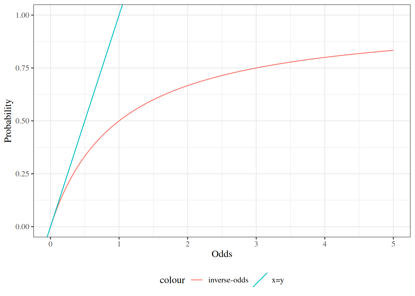
The inverse-odds function converts odds into their corresponding probabilities (Figure 2). Its domain of inputs is \(\omega\in [0,\infty)\) and its range of outputs is \(\pi\in [0,1]\).

I haven’t seen anyone give the inverse-odds function a concise name; maybe \(\operatorname{prob}()\) or \(\operatorname{prob}()\) or \(\operatorname{risk}()\)?

odds_inv <- function(omega) (1 + omega^-1)^-1
library(ggplot2)
ggplot() +
  geom_function(fun = odds_inv, aes(col = "inverse-odds")) +
  xlab("Odds") +
  ylab("Probability") +
  xlim(0, 5) +
  ylim(0, 1) +
  geom_abline(aes(intercept = 0, slope = 1, col = "x=y"))

Figure 2: The inverse odds function, \(\operatorname{invodds}\mathopen{}\left\{\omega\right\}\mathclose{}\)

Exercise 16 What probability corresponds to an odds of \(\omega= 1\), and what is the numerical difference between these two values?

SolutionSolution

Solution. \[ \begin{aligned} \pi &= \operatorname{invodds}\mathopen{}\left\{1\right\}\mathclose{} \\ &= \frac{1}{1+1} \\ &=\frac{1}{2} \\ &= .5 \end{aligned} \] \[ \begin{aligned} \omega- \pi&= 1 - .5 \\ &= .5 \end{aligned} \]

Lemma 1 (Simplified expression for inverse odds function)  

Equivalent expressions for the inverse odds function are:

\[ \begin{aligned} \operatorname{invodds}\mathopen{}\left\{\omega\right\}\mathclose{} &= \frac{1}{1+\omega^{-1}} \\ &= (1+\omega^{-1})^{-1} \end{aligned} \tag{13}\]

Exercise 17 Prove that Equation 13 is equivalent to Definition 11.

SolutionSolution

Solution 17. Analogous to Solution 13.

Lemma 2 (One minus inverse-odds) \[1 - \pi= \frac{1}{1+\omega}\]

ProofProof

Proof. By Theorem 6:

\[ \begin{aligned} 1 - \pi&= 1 - \frac{\omega}{1 + \omega} \\ &= \frac{{\color{red}{1+\omega}}}{1 + \omega} - \frac{{\color{teal}{\omega}}}{1 + \omega} \\ &= \frac{{\color{red}{(1+\omega)}} - {\color{teal}{\omega}}}{1 + \omega} \\ &= \frac{1 + \omega- \omega}{1 + \omega} \\ &= \frac{1}{1 + \omega} \end{aligned} \]

Corollary 5 (One plus odds in terms of non-event probability) \[1+\omega= \frac{1}{1-\pi}\]

1.3.3 Odds ratios

Now that we have defined odds, we can introduce another way of comparing event probabilities: odds ratios.

Definition 12 (Odds ratio) The odds ratio for two conditional odds, \(\omega_1\) and \(\omega_2\), is the ratio of those odds:

\[\theta(\omega_1, \omega_2) \stackrel{\text{def}}{=}\frac{\omega_1}{\omega_2}\]

There’s a 1:1 mapping between probability and odds, and according to that mapping, the odds are equal between two covariate patterns IF and ONLY IF the probabilities are also equal between those patterns.

An odds ratio is a ratio of odds. An odds is a ratio of probabilities, so odds ratios are ratios of ratios:

Theorem 7 (Odds ratio as a ratio of ratios) \[ \begin{aligned} \theta(\omega_1, \omega_2) &= \frac{\omega_1}{\omega_2} \\ &= \frac{\mathopen{}\left(\frac{\pi_1}{1-\pi_1}\right)\mathclose{}}{\mathopen{}\left(\frac{\pi_2}{1-\pi_2}\right)\mathclose{}} \end{aligned} \]

ProofProof

Proof. \[ \begin{aligned} \theta(\omega_1, \omega_2) &\stackrel{\text{def}}{=}\frac{\omega_1}{\omega_2} && \text{(@def-OR)} \\ &= \frac{\mathopen{}\left(\frac{\pi_1}{1-\pi_1}\right)\mathclose{}}{\mathopen{}\left(\frac{\pi_2}{1-\pi_2}\right)\mathclose{}} && \text{(@thm-prob-to-odds, applied to each odds)} \end{aligned} \]

Exm

Example 10 (The OC-MI odds ratio as a ratio of ratios) Using the MI risk estimates from Solution 1, \(\hat\pi(OC) = 13/5000\) and \(\hat\pi(\neg OC) = 7/10000\), Theorem 7 expresses the odds ratio as a ratio of the two odds, each of which is itself a ratio of probabilities:

\[ \begin{aligned} \theta(\omega(OC), \omega(\neg OC)) &\stackrel{\text{def}}{=}\frac{\omega(OC)}{\omega(\neg OC)} && \text{(@def-OR)} \\ &= \frac{\mathopen{}\left(\frac{\pi(OC)}{1-\pi(OC)}\right)\mathclose{}}{\mathopen{}\left(\frac{\pi(\neg OC)}{1-\pi(\neg OC)}\right)\mathclose{}} && \text{(@thm-prob-to-odds, applied to each odds)} \\ &= \frac{\mathopen{}\left(\frac{13/5000}{1 - 13/5000}\right)\mathclose{}}{\mathopen{}\left(\frac{7/10000}{1 - 7/10000}\right)\mathclose{}} && \text{(substituting the risk estimates)} \\ &= \frac{0.002607}{7.004903\times 10^{-4}} && \text{(computing each odds)} \\ &= 3.721361 && \text{(dividing)} \end{aligned} \]

Exm

Example 11 (Calculating odds ratios) In Example 1, the odds ratio for OC users versus OC-non-users is:

\[ \begin{aligned} \theta(\omega(OC), \omega(\neg OC)) &= \frac{\omega(OC)}{\omega(\neg OC)}\\ &= \frac{0.0026}{7\times 10^{-4}}\\ &= 3.714286\\ \end{aligned} \]

A shortcut for calculating odds ratio estimates

The general form of a two-by-two table is shown in Table 2.

Table 2: A generic 2x2 table

	Event	Non-Event	Total
Exposed	a	b	a+b
Non-exposed	c	d	c+d
Total	a+c	b+d	a+b+c+d

From this table, we have:

• \(\hat{\pi}(Event|Exposed) = a/(a+b)\)

• \(\hat{\pi}(\neg Event|Exposed) = b/(a+b)\)

• \(\hat{\omega}(Event|Exposed) = \frac{\frac{a}{a+b}}{\frac{b}{a+b}}=\frac{a}{b}\)

• \(\hat{\omega}(Event|\neg Exposed) = \frac{c}{d}\) (see Exercise 18)

• \(\theta_{\omega}(Exposed,\neg Exposed) = \frac{\frac{a}{b}}{\frac{c}{d}} = \frac{ad}{bc}\)

Exercise 18 Given Table 2, show that \(\hat{\omega}(Event|\neg Exposed) = \frac{c}{d}\).

Properties of odds ratios

Odds ratios have a special property: we can swap a covariate with the outcome, and the odds ratio remains the same.

Theorem 8 (Odds ratios are reversible) For any two events \(A\), \(B\):

\[\theta_{\omega}(A|B) = \theta_{\omega}(B|A)\]

ProofProof

Proof. Using Definition 12, Definition 8, the law of conditional probability, and the definition of conditional probability:

\[ \begin{aligned} \theta_{\omega}(A|B) &\stackrel{\text{def}}{=}\frac{\omega(A|B)}{\omega(A|\neg B)} && \text{(definition of odds ratio)} \\ &= \frac {\mathopen{}\left(\frac{\operatorname{p}(A|B)}{\operatorname{p}(\neg A|B)}\right)\mathclose{}} {\mathopen{}\left(\frac{\operatorname{p}(A|\neg B)}{\operatorname{p}(\neg A| \neg B)}\right)\mathclose{}} && \text{(definition of conditional odds)} \\ &= \mathopen{}\left(\frac{\operatorname{p}(A|B)}{\operatorname{p}(\neg A|B)}\right)\mathclose{} \mathopen{}\left(\frac{\operatorname{p}(A|\neg B)}{\operatorname{p}(\neg A| \neg B)}\right)^{-1}\mathclose{} && \text{(division is multiplication by the reciprocal)} \\ &= \mathopen{}\left(\frac{\operatorname{p}(A|B)}{\operatorname{p}(\neg A|B)}\right)\mathclose{} \mathopen{}\left(\frac{\operatorname{p}(\neg A| \neg B)}{\operatorname{p}(A|\neg B)}\right)\mathclose{} && \text{(the reciprocal of a fraction flips it)} \\ &= \mathopen{}\left(\frac{\operatorname{p}(A|B)}{\operatorname{p}(\neg A|B)} \cdot\frac{\operatorname{p}(B)}{\operatorname{p}(B)}\right)\mathclose{} \mathopen{}\left(\frac{\operatorname{p}(\neg A| \neg B)}{\operatorname{p}(A|\neg B)} \cdot\frac{\operatorname{p}(\neg B)}{\operatorname{p}(\neg B)}\right)\mathclose{} && \text{(multiply each factor by 1)} \\ &= \mathopen{}\left(\frac{\operatorname{p}(A,B)}{\operatorname{p}(\neg A,B)}\right)\mathclose{} \mathopen{}\left(\frac{\operatorname{p}(\neg A, \neg B)}{\operatorname{p}(A, \neg B)}\right)\mathclose{} && \text{(law of conditional probability, in each of the four terms)} \\ &= \mathopen{}\left(\frac{\operatorname{p}(B,A)}{{\color{red}{\operatorname{p}(B,\neg A)}}}\right)\mathclose{} \mathopen{}\left(\frac{\operatorname{p}(\neg B, \neg A)}{{\color{teal}{\operatorname{p}(\neg B, A)}}}\right)\mathclose{} && \text{(joint probabilities are symmetric in their arguments)} \\ &= \mathopen{}\left(\frac{\operatorname{p}(B,A)}{{\color{teal}{\operatorname{p}(\neg B, A)}}}\right)\mathclose{} \mathopen{}\left(\frac{\operatorname{p}(\neg B, \neg A)}{{\color{red}{\operatorname{p}(B,\neg A)}}}\right)\mathclose{} && \text{(swap the two highlighted denominators)} \\ &= \mathopen{}\left(\frac{\operatorname{p}(B,A) / \operatorname{p}(A)}{\operatorname{p}(\neg B, A) / \operatorname{p}(A)}\right)\mathclose{} \mathopen{}\left(\frac{\operatorname{p}(\neg B, \neg A) / \operatorname{p}(\neg A)}{\operatorname{p}(B,\neg A) / \operatorname{p}(\neg A)}\right)\mathclose{} && \text{(divide the top and bottom of each factor by the same quantity)} \\ &= \mathopen{}\left(\frac{\operatorname{p}(B|A)}{\operatorname{p}(\neg B|A)}\right)\mathclose{} \mathopen{}\left(\frac{\operatorname{p}(\neg B| \neg A)}{\operatorname{p}(B|\neg A)}\right)\mathclose{} && \text{(definition of conditional probability, in each of the four terms)} \\ &= \mathopen{}\left(\frac{\operatorname{p}(B|A)}{\operatorname{p}(\neg B|A)}\right)\mathclose{} \mathopen{}\left(\frac{\operatorname{p}(B|\neg A)}{\operatorname{p}(\neg B| \neg A)}\right)^{-1}\mathclose{} && \text{(a flipped fraction is the reciprocal of the original)} \\ &= \frac {\mathopen{}\left(\frac{\operatorname{p}(B|A)}{\operatorname{p}(\neg B|A)}\right)\mathclose{}} {\mathopen{}\left(\frac{\operatorname{p}(B|\neg A)}{\operatorname{p}(\neg B| \neg A)}\right)\mathclose{}} && \text{(multiplication by the reciprocal is division)} \\ &= \frac{\omega(B|A)}{\omega(B|\neg A)} && \text{(definition of conditional odds)} \\ &\stackrel{\text{def}}{=}\theta_{\omega}(B|A) && \text{(definition of odds ratio)} \end{aligned} \]

Exm

Example 12 (Reversibility of the OC-MI odds ratio) Theorem 8 says \(\theta_{\omega}(MI|OC) = \theta_{\omega}(OC|MI)\): we can swap the roles of the outcome (MI) and the covariate (OC use) without changing the odds ratio. We can confirm this equality numerically using the counts from Example 1.

The disease odds ratio (the odds of MI, comparing OC users to non-users) is:

\[ \begin{aligned} \hat{\theta_{\omega}}(MI|OC) &\stackrel{\text{def}}{=}\frac{\hat{\omega}(MI|OC)}{\hat{\omega}(MI|\neg OC)} && \text{(@def-OR, applied to the estimated odds)} \\ &= \frac{13/4987}{7/9993} && \text{(@thm-est-odds: estimated odds = events/non-events; counts from @exm-oc-mi)} \\ &= \frac{0.002607}{7.004903\times 10^{-4}} && \text{(dividing within each OC-use group)} \\ &= 3.721361 && \text{(dividing)} \end{aligned} \]

The exposure odds ratio (the odds of OC use, comparing MI cases to non-cases) is:

\[ \begin{aligned} \hat{\theta_{\omega}}(OC|MI) &\stackrel{\text{def}}{=}\frac{\hat{\omega}(OC|MI)}{\hat{\omega}(OC|\neg MI)} && \text{(@def-OR, applied to the estimated odds)} \\ &= \frac{13/7}{4987/9993} && \text{(@thm-est-odds: estimated odds = events/non-events; counts from @exm-oc-mi)} \\ &= \frac{1.857143}{0.499049} && \text{(dividing within each MI-status group)} \\ &= 3.721361 && \text{(dividing)} \end{aligned} \]

Both equal 3.721361, confirming Theorem 8.

Exercise 19 For Table 2, show that \(\hat{\theta_{\omega}}(Exposed, Unexposed) = \hat{\theta_{\omega}}(Event, \neg Event)\).

Conditional odds ratios have the same reversibility property:

Theorem 9 (Conditional odds ratios are reversible) For any three events \(A\), \(B\), \(C\):

\[\theta_{\omega}(A|B,C) = \theta_{\omega}(B|A,C)\]

ProofProof

Proof. Apply the same steps as for Theorem 8, inserting \(C\) into the conditions (RHS of \(|\)) of every expression.

Exm

Example 13 (Reversibility within age strata in the WCGS data) Theorem 9 says a conditional odds ratio is also reversible: \(\theta_{\omega}(A|B,C) = \theta_{\omega}(B|A,C)\). We can illustrate this equality using data from the Western Collaborative Group Study (wcgs) (Rosenman et al. 1975), a prospective cohort study of coronary heart disease (CHD) in 3,154 men aged 39–59, which classified each participant’s behavioral pattern as Type A (urgent, competitive) or Type B (relaxed). For this example, we take the covariate \(B\) to be behavioral pattern (Type A versus Type B), the outcome \(A\) to be CHD by 1969, and the conditioning event \(C\) to be an age stratum.

Among participants under 50, the disease odds ratio (the odds of CHD, comparing Type A to Type B) is 2.212757, and the exposure odds ratio (the odds of Type A, comparing CHD cases to non-cases) is 2.212757; the two agree, as Theorem 9 requires.

Among participants aged 50 or older, the disease and exposure odds ratios are 2.30791 and 2.30791, which likewise agree.

Odds Ratios vs Probability (Risk) Ratios

When the outcome is rare (i.e., its probability is small) for both groups being compared in an odds ratio, the odds of the outcome will be similar to the probability of the outcome, and thus the risk ratio will be similar to the odds ratio.

Case 1: rare events

For rare events, odds ratios and probability (a.k.a. risk, a.k.a. prevalence) ratios will be close:

\[\pi_1 = .01\] \[\pi_2 = .02\]

pi1 <- .01
pi2 <- .02
pi2 / pi1
#> [1] 2
odds(pi2) / odds(pi1)
#> [1] 2.02041

Exm

Example 14 In Example 1, the outcome is rare for both OC and non-OC participants, so the odds for both groups are similar to the corresponding probabilities, and the odds ratio is similar the risk ratio.

Case 2: frequent events

\[\pi_1 = .4\]

\[\pi_2 = .5\]

For more frequently-occurring outcomes, this won’t be the case:

pi1 <- .4
pi2 <- .5
pi2 / pi1
#> [1] 1.25
odds(pi2) / odds(pi1)
#> [1] 1.5

The relationship between the two spot-checks is captured by a simple algebraic identity:

Theorem 10 (Odds ratio as risk ratio times a correction factor) For two probabilities \(\pi_1\) and \(\pi_2\), the odds ratio equals the risk ratio times a correction factor:

\[\theta(\omega_1, \omega_2) = \rho(\pi_1, \pi_2) \cdot \frac{1-\pi_2}{1-\pi_1} \tag{14}\]

When \(\pi_1\) and \(\pi_2\) are both small, the correction factor \(\frac{1-\pi_2}{1-\pi_1}\) is close to 1, so the odds ratio is close to the risk ratio.

ProofProof

Proof. \[ \begin{aligned} \theta(\omega_1, \omega_2) &\stackrel{\text{def}}{=}\frac{\omega_1}{\omega_2} && \text{(@def-OR)} \\ &= \frac{\mathopen{}\left(\frac{\pi_1}{1-\pi_1}\right)\mathclose{}}{\mathopen{}\left(\frac{\pi_2}{1-\pi_2}\right)\mathclose{}} && \text{(@thm-prob-to-odds, applied to each odds)} \\ &= \frac{\pi_1}{\pi_2} \cdot \frac{1-\pi_2}{1-\pi_1} && \text{(rearranging the compound fraction)} \\ &= \rho(\pi_1, \pi_2) \cdot \frac{1-\pi_2}{1-\pi_1} && \text{(@def-RR)} \end{aligned} \]

Exm

Example 15 (The correction factor in the two spot-checks) Theorem 10 explains the two spot-checks preceding it.

In Case 1 (rare events), take \(\pi_1 = 0.02\) and \(\pi_2 = 0.01\). The correction factor \(\frac{1-\pi_2}{1-\pi_1} = 1.010204\) is close to 1, so the odds ratio (2.020408) is close to the risk ratio (2).

In Case 2 (frequent events), take \(\pi_1 = 0.5\) and \(\pi_2 = 0.4\). The correction factor \(\frac{1-\pi_2}{1-\pi_1} = 1.2\) is farther from 1, so the odds ratio (1.5) and risk ratio (1.25) diverge.

Figure 3 compares risk differences, risk ratios, and odds ratios as functions of the underlying probabilities being compared.

if (run_graphs) {
  RD <- function(p1, p2) p2 - p1
  RR <- function(p1, p2) p2 / p1
  odds <- function(p) p / (1 - p)
  OR <- function(p1, p2) odds(p2) / odds(p1)
  OR_minus_RR <- function(p1, p2) OR(p2, p1) - RR(p2, p1)

  n_ticks <- 201
  probs <- seq(.001, .99, length.out = n_ticks)
  RD_mat <- outer(probs, probs, RD)
  RR_mat <- outer(probs, probs, RR)
  OR_mat <- outer(probs, probs, OR)

  opacity <- .3
  z_min <- -1
  z_max <- 5
  plotly::plot_ly(
    x = ~probs,
    y = ~probs
  ) |>
    plotly::add_surface(
      z = ~ t(RD_mat),
      contours = list(
        z = list(
          show = TRUE,
          start = -1,
          end = 1,
          size = .1
        )
      ),
      name = "Risk Difference",
      showscale = FALSE,
      opacity = opacity,
      colorscale = list(c(0, 1), c("green", "green"))
    ) |>
    plotly::add_surface(
      opacity = opacity,
      colorscale = list(c(0, 1), c("red", "red")),
      z = ~ t(RR_mat),
      contours = list(
        z = list(
          show = TRUE,
          start = z_min,
          end = z_max,
          size = .2
        )
      ),
      showscale = FALSE,
      name = "Risk Ratio"
    ) |>
    plotly::add_surface(
      opacity = opacity,
      colorscale = list(c(0, 1), c("blue", "blue")),
      z = ~ t(OR_mat),
      contours = list(
        z = list(
          show = TRUE,
          start = z_min,
          end = z_max,
          size = .2
        )
      ),
      showscale = FALSE,
      name = "Odds Ratio"
    ) |>
    plotly::layout(
      scene = list(
        xaxis = list(
          # type = "log",
          title = "reference group probability"
        ),
        yaxis = list(
          # type = "log",
          title = "comparison group probability"
        ),
        zaxis = list(
          # type = "log",
          range = c(z_min, z_max),
          title = "comparison metric"
        ),
        camera = list(eye = list(x = -1.25, y = -1.25, z = 0.5)),
        aspectratio = list(x = .9, y = .8, z = 0.7)
      )
    )
}

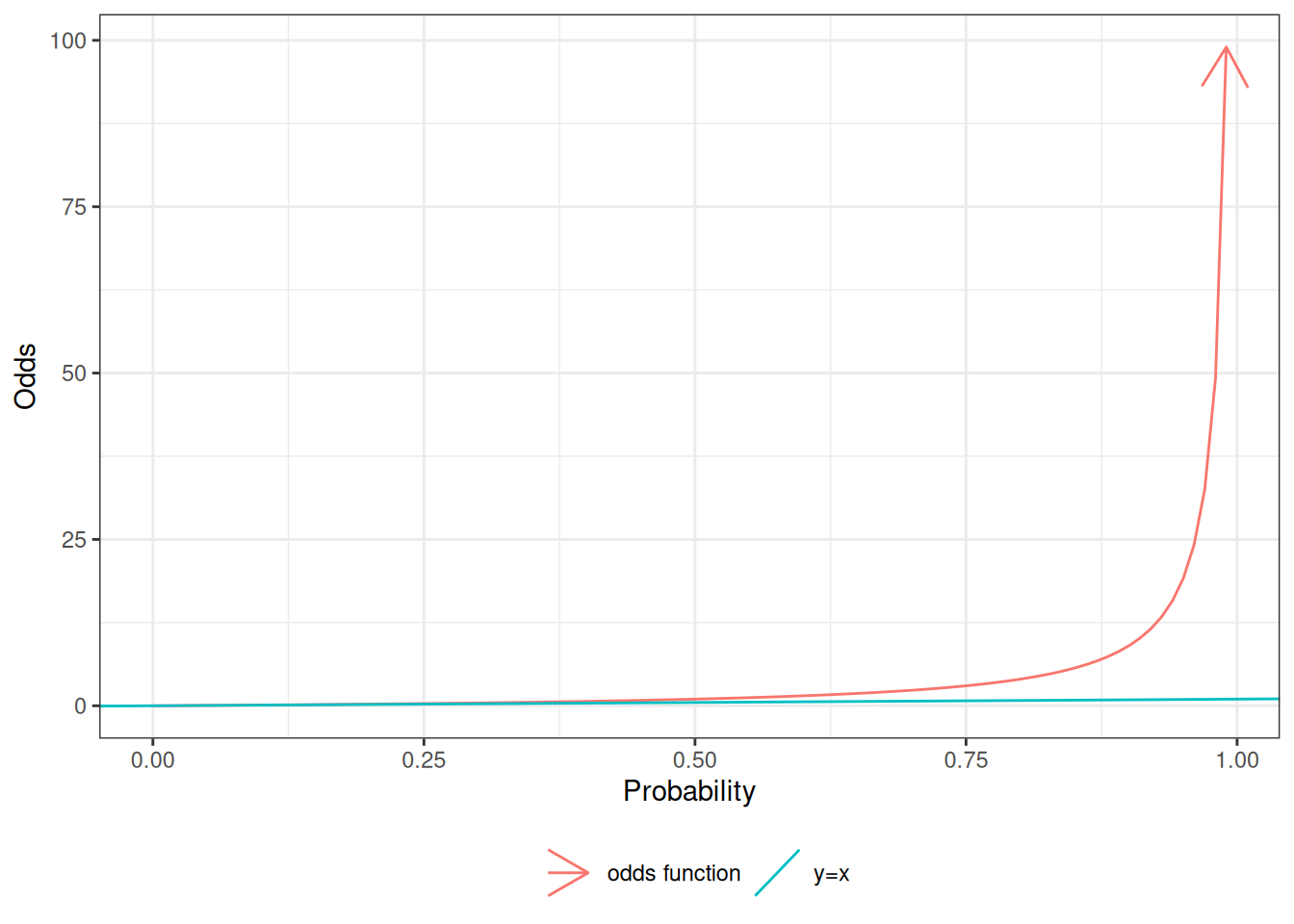
Figure 3: Graph of risk difference, risk ratio, and odds ratio

Testing whether an odds ratio = 1 is equivalent to testing whether the corresponding risk ratio = 1, and also equivalent to testing whether the risk difference = 0. Therefore, in hypothesis testing, if the null hypothesis is no effect, then we can shift between RD, RR, and OR. But when we’re talking about point estimates and CIs, we need to limit our conclusions to the effect measure(s) that we actually estimated, because the sizes of RDs, RRs, and ORs don’t have a simple relationship to each other, except when \(\pi_1=\pi_2\) (as shown by Figure 3).

Odds Ratios in Case-Control Studies

Table 1 simulates a follow-up study in which two populations were followed and the number of MI’s was observed. The risks are \(P(MI|OC)\) and \(P(MI|\neg OC)\) and we can estimate these risks from the data.

But suppose we had a case-control study in which we had 100 women with MI and selected a comparison group of 100 women without MI (matched as groups on age, etc.). Then MI is not random, and we cannot compute P(MI|OC) and we cannot compute the risk ratio. However, the odds ratio can be computed.

Definition 13 (Disease odds ratio) For a disease \(D\) and an exposure \(E\), the disease odds ratio is the odds of disease in the exposed group divided by the odds of disease in the unexposed group:

\[\theta_{\omega}(D|E) \stackrel{\text{def}}{=}\frac{\omega(D|E)}{\omega(D|\neg E)}\]

In a case-control study, disease status is not random, so we cannot validly compute or use the separate parts \(\omega(D|E)\) and \(\omega(D|\neg E)\) of the disease odds ratio.

Definition 14 (Exposure odds ratio) For a disease \(D\) and an exposure \(E\), the exposure odds ratio is the odds of exposure in the diseased group divided by the odds of exposure in the non-diseased group:

\[\theta_{\omega}(E|D) \stackrel{\text{def}}{=}\frac{\omega(E|D)}{\omega(E|\neg D)}\]

We can still validly compute and use the exposure odds ratio, because exposure can be treated as random.

Exm

Example 16 (Exposure odds ratio in the OC-MI study) For the OC-MI study, the estimated exposure odds ratio is:

\[ \hat{\theta_{\omega}}(OC|MI) = \frac{\hat{\omega}(OC|MI)}{\hat{\omega}(OC|\neg MI)} \]

And these two odds ratios, \(\hat{\theta_{\omega}}(MI|OC)\) and \(\hat{\theta_{\omega}}(OC|MI)\), are mathematically equivalent, as we saw in Section 1.3.3.2:

\[\hat{\theta_{\omega}}(MI|OC) = \hat{\theta_{\omega}}(OC|MI)\]

Exercise 20 Calculate the odds ratio of MI with respect to OC use, assuming that Table 1 comes from a case-control study. Confirm that the result is the same as in Example 11.

SolutionSolution

Solution.

tbl_oc_mi |> pander::pander()

Table 3: Simulated data from study of oral contraceptive use and heart attack risk

OC	MI	No MI	Total
OC use	13	4,987	5,000
No OC use	7	9,993	10,000
Total	20	14,980	15,000

• \(\omega(OC|MI) = P(OC|MI)/(1 - P(OC|MI)) = \frac{13}{7} = 1.857143\)

• \(\omega(OC|\neg MI) = P(OC|\neg MI)/(1 - P(OC|\neg MI)) = \frac{4987}{9993} = 0.499049\)

• \(\theta_{\omega}(OC|MI) = \frac{\omega(OC|MI)}{\omega(OC|\neg MI)} = \frac{13/7}{4987/9993} = 3.721361\)

This odds-ratio estimate is the same one we calculated in Example 11.

Odds Ratios in Cross-Sectional Studies

• If a cross-sectional study is a uniform probability sample of a population (which it rarely is), then we can estimate prevalence (sometimes called “prevalence risk” or just “risk”) using standard methods (Lee 1994), and we can thus also estimate prevalence differences, prevalence ratios, and prevalence odds ratios comparing sub-populations.

• If the cross-sectional study is a stratified probability sample, then we can estimate prevalence, prevalence differences, prevalence ratios, and prevalence odds ratios using specialized methods for complex surveys (Lumley 2010).

• If the study has sampling biases that we cannot adjust for with survey weights, such as in a convenience sample, then we need to treat it in the same way as a case-control study, and we cannot validly estimate prevalence, prevalence differences, or prevalence ratios; we can only validly estimate prevalence odds ratios.

1.4 The logit and expit functions

1.4.1 The logit function

Definition 15 (log-odds)  

If \(\omega\) is the odds of an event \(A\), then the log-odds of \(A\), which we will represent by \(\eta\) (“eta”), is the natural logarithm of the odds of \(A\):

\[\eta\stackrel{\text{def}}{=}\operatorname{log}\mathopen{}\left\{\omega\right\}\mathclose{} \tag{15}\]

Theorem 11 (Log-odds as a function of probability) If \(\pi\) is the probability of an event \(A\), \(\omega\) is the corresponding odds of \(A\), and \(\eta\) is the corresponding log-odds of \(A\), then:

\[\eta= \operatorname{log}\mathopen{}\left\{\frac{\pi}{1-\pi}\right\}\mathclose{} \tag{16}\]

ProofProof

Proof. Using Definition 15 and Theorem 2:

\[ \begin{aligned} \eta&\stackrel{\text{def}}{=}\operatorname{log}\mathopen{}\left\{\omega\right\}\mathclose{} && \text{(definition of log-odds)} \\ &= \operatorname{log}\mathopen{}\left\{\frac{\pi}{1-\pi}\right\}\mathclose{} && \text{(odds as a function of probability)} \end{aligned} \]

Definition 16 (logit function)  

The logit function of a probability \(\pi\) is the natural logarithm of the odds function of \(\pi\):

\[\operatorname{logit}(\pi) \stackrel{\text{def}}{=}\operatorname{log}\mathopen{}\left\{\operatorname{odds}\mathopen{}\left\{\pi\right\}\mathclose{}\right\}\mathclose{}\]

The logit function is a composite function.

Exercise 21 (Compose the logit function) Mathematically expand the definition of the logit function.

SolutionSolution (Compose the logit function)

Solution 18 (Compose the logit function).

Theorem 12 (Expanded expression for logit) \[\operatorname{logit}(\pi) = \operatorname{log}\mathopen{}\left\{\frac{\pi}{1-\pi}\right\}\mathclose{} \tag{17}\]

ProofProof

Proof. Using Definition 16 and Definition 10:

\[ \begin{aligned} \operatorname{logit}(\pi) &\stackrel{\text{def}}{=}\operatorname{log}\mathopen{}\left\{\operatorname{odds}\mathopen{}\left\{\pi\right\}\mathclose{}\right\}\mathclose{} && \text{(definition of logit)} \\ &= \operatorname{log}\mathopen{}\left\{\frac{\pi}{1-\pi}\right\}\mathclose{} && \text{(definition of the odds function)} \end{aligned} \]

Corollary 6 (Log-odds via the logit function) If \(\pi\) is the probability of an event \(A\) and \(\eta\) is the corresponding log-odds of \(A\), then:

\[\eta= \operatorname{logit}\mathopen{}\left\{\pi\right\}\mathclose{}\]

ProofProof

Proof. Using Theorem 11 and Theorem 12:

\[ \begin{aligned} \eta&= \operatorname{log}\mathopen{}\left\{\frac{\pi}{1-\pi}\right\}\mathclose{} && \text{(log-odds as a function of probability)} \\ &= \operatorname{logit}\mathopen{}\left\{\pi\right\}\mathclose{} && \text{(expanded expression for logit, read right-to-left)} \end{aligned} \]

Exm

Example 17 (Log-odds of an event with probability 0.75) Suppose the probability of an event \(A\) is \(\pi= 0.75\). Then, by Theorem 2, the corresponding odds of \(A\) are \(\omega= \frac{0.75}{1-0.75} = \frac{0.75}{0.25} = 3\), and by Corollary 6 and Theorem 12, the corresponding log-odds of \(A\) are:

\[ \begin{aligned} \eta= \operatorname{logit}\mathopen{}\left\{0.75\right\}\mathclose{} &= \operatorname{log}\mathopen{}\left\{\frac{0.75}{1-0.75}\right\}\mathclose{} && \text{(expanded expression for logit)} \\ &= \operatorname{log}\mathopen{}\left\{\frac{0.75}{0.25}\right\}\mathclose{} && \text{(subtract: } 1 - 0.75 = 0.25\text{)} \\ &= \operatorname{log}\mathopen{}\left\{3\right\}\mathclose{} && \text{(divide: } 0.75 / 0.25 = 3\text{)} \\ &\approx 1.0986 && \text{(evaluate the natural logarithm)} \end{aligned} \]

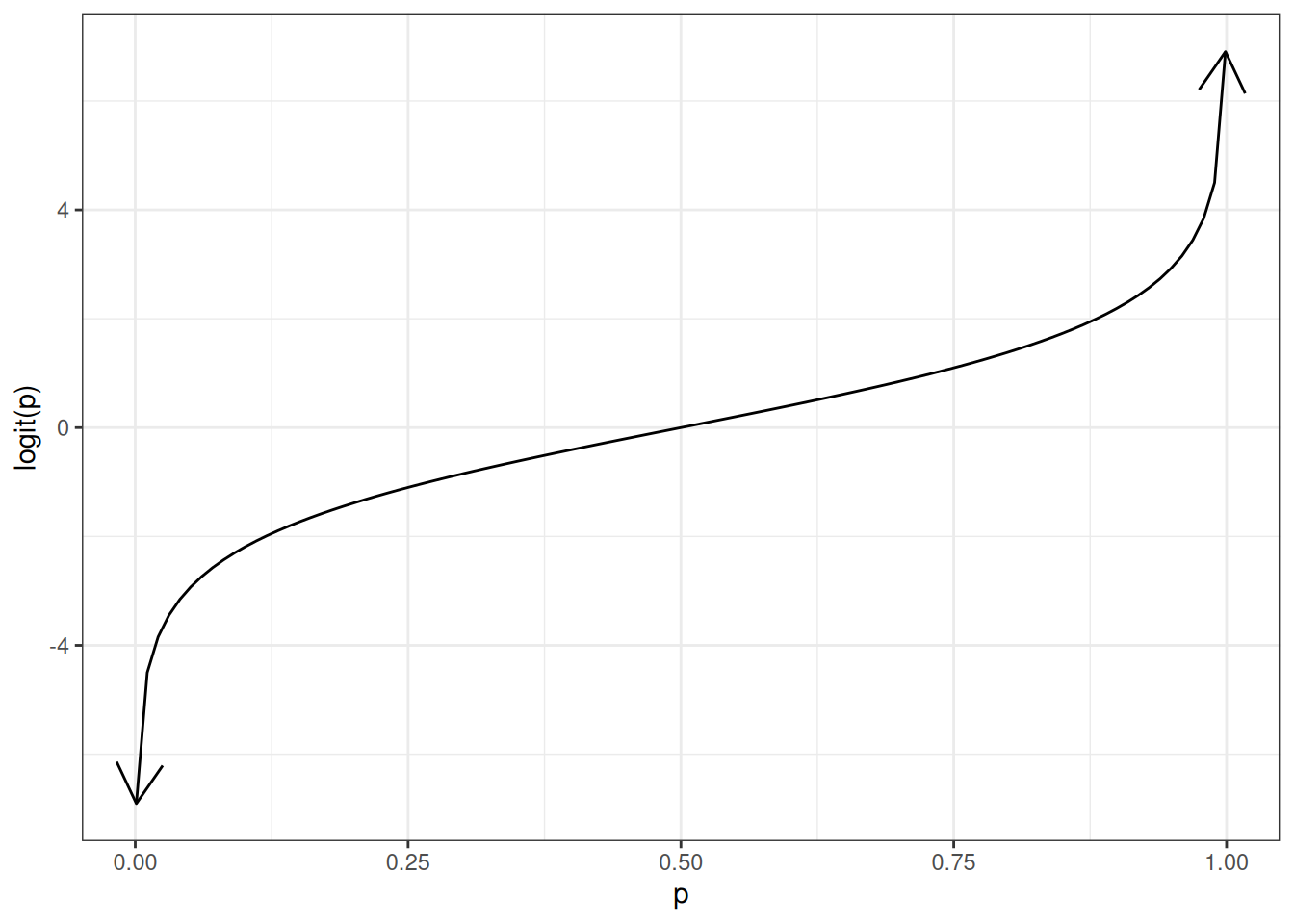
Figure 4 shows the shape of the \(\operatorname{logit}()\) function.

odds <- function(pi) pi / (1 - pi)

logit <- function(p) log(odds(p))

library(ggplot2)
logit_plot <-
  ggplot() +
  geom_function(
    fun = logit,
    arrow = arrow(ends = "both")
  ) +
  xlim(.001, .999) +
  ylab("logit(p)") +
  xlab("p") +
  theme_bw()
print(logit_plot)

Figure 4: The logit function

1.4.2 The expit function

Lemma 3 (Odds from log-odds)  

If \(\omega\) is the odds of an event \(A\) and \(\eta\) is the corresponding log-odds of \(A\), then:

\[\omega= \operatorname{exp}\mathopen{}\left\{\eta\right\}\mathclose{}\]

ProofProof

Proof. Starting from Definition 15, we solve for \(\omega\):

\[ \begin{aligned} \eta&\stackrel{\text{def}}{=}\operatorname{log}\mathopen{}\left\{\omega\right\}\mathclose{} && \text{(definition of log-odds)} \\ \operatorname{exp}\mathopen{}\left\{\eta\right\}\mathclose{} &= \operatorname{exp}\mathopen{}\left\{\operatorname{log}\mathopen{}\left\{\omega\right\}\mathclose{}\right\}\mathclose{} && \text{(exponentiate both sides)} \\ \operatorname{exp}\mathopen{}\left\{\eta\right\}\mathclose{} &= \omega && \text{(the exponential function inverts the natural logarithm)} \\ \omega&= \operatorname{exp}\mathopen{}\left\{\eta\right\}\mathclose{} && \text{(swap the two sides of the equation)} \end{aligned} \]

Theorem 13 (Probability as a function of log-odds)  

If \(\pi\) is the probability of an event \(A\), \(\omega\) is the corresponding odds of \(A\), and \(\eta\) is the corresponding log-odds of \(A\), then:

\[\pi= \frac{\operatorname{exp}\mathopen{}\left\{\eta\right\}\mathclose{}}{1+\operatorname{exp}\mathopen{}\left\{\eta\right\}\mathclose{}}\]

ProofProof

Proof. Using Theorem 6 and Lemma 3:

\[ \begin{aligned} \pi&= \frac{\omega}{1+\omega} && \text{(probability as a function of odds)} \\ &= \frac{\operatorname{exp}\mathopen{}\left\{\eta\right\}\mathclose{}}{1+\operatorname{exp}\mathopen{}\left\{\eta\right\}\mathclose{}} && \text{(substitute } \omega= \operatorname{exp}\mathopen{}\left\{\eta\right\}\mathclose{} \text{ in both places)} \end{aligned} \]

Definition 17 (expit, logistic, inverse-logit) The expit function of a log-odds \(\eta\), also known as the inverse-logit function or logistic function, is the inverse-odds of the exponential of \(\eta\):

\[\operatorname{expit}(\eta) \stackrel{\text{def}}{=}\operatorname{invodds}\mathopen{}\left\{\operatorname{exp}\mathopen{}\left\{\eta\right\}\mathclose{}\right\}\mathclose{}\]

Theorem 14 (Expressions for expit function) \[ \begin{aligned} \operatorname{expit}(\eta) &= \frac{\operatorname{exp}\mathopen{}\left\{\eta\right\}\mathclose{}}{1+\operatorname{exp}\mathopen{}\left\{\eta\right\}\mathclose{}} \\ &= \frac{1}{1 + \operatorname{exp}\mathopen{}\left\{-\eta\right\}\mathclose{}} \\ &= (1 + \operatorname{exp}\mathopen{}\left\{-\eta\right\}\mathclose{})^{-1} \end{aligned} \]

ProofProof

Proof. For the first expression, apply Definition 17 and then Definition 11:

\[ \begin{aligned} \operatorname{expit}(\eta) &\stackrel{\text{def}}{=}\operatorname{invodds}\mathopen{}\left\{\operatorname{exp}\mathopen{}\left\{\eta\right\}\mathclose{}\right\}\mathclose{} && \text{(definition of expit)} \\ &= \frac{\operatorname{exp}\mathopen{}\left\{\eta\right\}\mathclose{}}{1+\operatorname{exp}\mathopen{}\left\{\eta\right\}\mathclose{}} && \text{(definition of inverse-odds, applied to } \omega= \operatorname{exp}\mathopen{}\left\{\eta\right\}\mathclose{}\text{)} \end{aligned} \]

For the second and third expressions, apply Definition 17 and then Lemma 1:

\[ \begin{aligned} \operatorname{expit}(\eta) &\stackrel{\text{def}}{=}\operatorname{invodds}\mathopen{}\left\{\operatorname{exp}\mathopen{}\left\{\eta\right\}\mathclose{}\right\}\mathclose{} && \text{(definition of expit)} \\ &= \frac{1}{1+\mathopen{}\left(\operatorname{exp}\mathopen{}\left\{\eta\right\}\mathclose{}\right)^{-1}\mathclose{}} && \text{(simplified inverse-odds, applied to } \omega= \operatorname{exp}\mathopen{}\left\{\eta\right\}\mathclose{}\text{)} \\ &= \frac{1}{1 + \operatorname{exp}\mathopen{}\left\{-\eta\right\}\mathclose{}} && \text{(negative-exponent rule: } \mathopen{}\left(\operatorname{exp}\mathopen{}\left\{x\right\}\mathclose{}\right)^{-1}\mathclose{} = \operatorname{exp}\mathopen{}\left\{-x\right\}\mathclose{}\text{)} \\ &= \mathopen{}\left(1 + \operatorname{exp}\mathopen{}\left\{-\eta\right\}\mathclose{}\right)^{-1}\mathclose{} && \text{(rewrite the reciprocal as a } -1 \text{ power)} \end{aligned} \]

Theorem 15 (Probability via the expit function) If \(\pi\) is the probability of an event \(A\), \(\omega\) is the corresponding odds of \(A\), and \(\eta\) is the corresponding log-odds of \(A\), then:

\[\pi= \operatorname{expit}\mathopen{}\left\{\eta\right\}\mathclose{}\]

ProofProof

Proof. Using Theorem 13 and Theorem 14:

\[ \begin{aligned} \pi&= \frac{\operatorname{exp}\mathopen{}\left\{\eta\right\}\mathclose{}}{1+\operatorname{exp}\mathopen{}\left\{\eta\right\}\mathclose{}} && \text{(probability as a function of log-odds)} \\ &= \operatorname{expit}\mathopen{}\left\{\eta\right\}\mathclose{} && \text{(first expression for expit, read right-to-left)} \end{aligned} \]

Exm

Example 18 (Probability of an event with log-odds \(\operatorname{log}\mathopen{}\left\{3\right\}\mathclose{}\)) In Example 17, a probability of \(\pi= 0.75\) corresponded to a log-odds of \(\eta= \operatorname{log}\mathopen{}\left\{3\right\}\mathclose{} \approx 1.0986\). By Theorem 15 and Theorem 14, the expit function recovers the probability from that log-odds:

\[ \begin{aligned} \pi= \operatorname{expit}\mathopen{}\left\{\operatorname{log}\mathopen{}\left\{3\right\}\mathclose{}\right\}\mathclose{} &= \frac{\operatorname{exp}\mathopen{}\left\{\operatorname{log}\mathopen{}\left\{3\right\}\mathclose{}\right\}\mathclose{}}{1+\operatorname{exp}\mathopen{}\left\{\operatorname{log}\mathopen{}\left\{3\right\}\mathclose{}\right\}\mathclose{}} && \text{(first expression for expit)} \\ &= \frac{3}{1 + 3} && \text{(the exponential inverts the natural logarithm: } \operatorname{exp}\mathopen{}\left\{\operatorname{log}\mathopen{}\left\{3\right\}\mathclose{}\right\}\mathclose{} = 3\text{)} \\ &= \frac{3}{4} && \text{(add: } 1 + 3 = 4\text{)} \\ &= 0.75 && \text{(divide: } 3/4 = 0.75\text{)} \end{aligned} \]

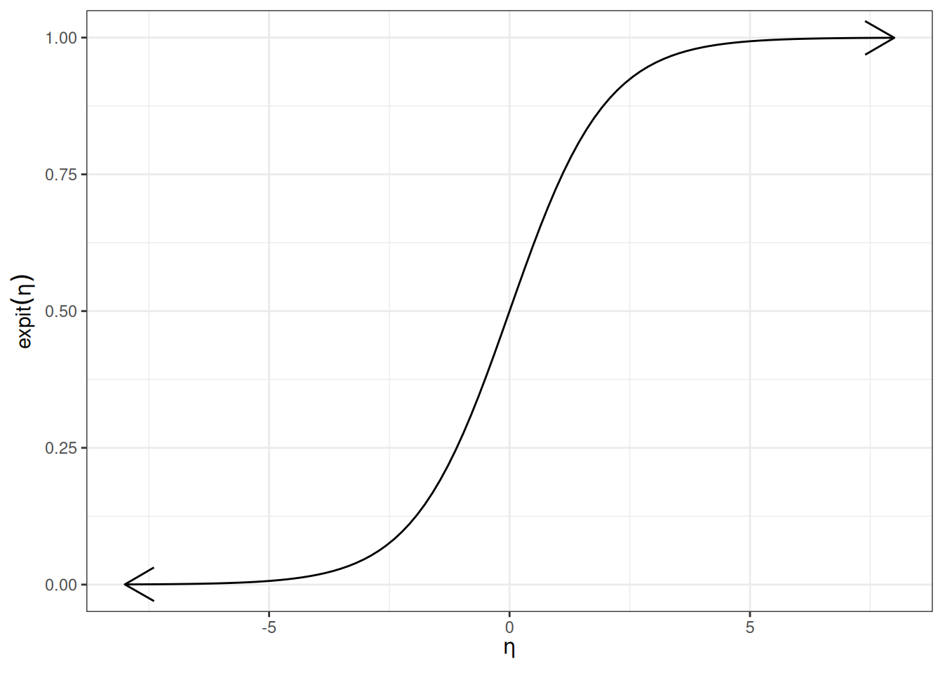
Figure 5 graphs the expit function.

expit <- function(eta) {
  exp(eta) / (1 + exp(eta))
}
library(ggplot2)
expit_plot <-
  ggplot() +
  geom_function(
    fun = expit,
    arrow = arrow(ends = "both")
  ) +
  xlim(-8, 8) +
  ylim(0, 1) +
  ylab(expression(expit(eta))) +
  xlab(expression(eta)) +
  theme_bw()
print(expit_plot)

Figure 5: The expit function

Theorem 16 (logit and expit are each others’ inverses) \[\operatorname{logit}\mathopen{}\left\{\operatorname{expit}\mathopen{}\left\{\eta\right\}\mathclose{}\right\}\mathclose{} = \eta\]

\[\operatorname{expit}\mathopen{}\left\{\operatorname{logit}\mathopen{}\left\{\pi\right\}\mathclose{}\right\}\mathclose{} = \pi\]

ProofProof

Proof. First, we show that \(\operatorname{logit}\mathopen{}\left\{\operatorname{expit}\mathopen{}\left\{\eta\right\}\mathclose{}\right\}\mathclose{} = \eta\), using Definition 16, Definition 17, and Corollary 4:

\[ \begin{aligned} \operatorname{logit}\mathopen{}\left\{\operatorname{expit}\mathopen{}\left\{\eta\right\}\mathclose{}\right\}\mathclose{} &\stackrel{\text{def}}{=}\operatorname{log}\mathopen{}\left\{\operatorname{odds}\mathopen{}\left\{\operatorname{expit}\mathopen{}\left\{\eta\right\}\mathclose{}\right\}\mathclose{}\right\}\mathclose{} && \text{(definition of logit, applied to } \pi= \operatorname{expit}\mathopen{}\left\{\eta\right\}\mathclose{}\text{)} \\ &= \operatorname{log}\mathopen{}\left\{\operatorname{odds}\mathopen{}\left\{\operatorname{invodds}\mathopen{}\left\{\operatorname{exp}\mathopen{}\left\{\eta\right\}\mathclose{}\right\}\mathclose{}\right\}\mathclose{}\right\}\mathclose{} && \text{(definition of expit)} \\ &= \operatorname{log}\mathopen{}\left\{\operatorname{exp}\mathopen{}\left\{\eta\right\}\mathclose{}\right\}\mathclose{} && \text{(the odds function inverts the inverse-odds function)} \\ &= \eta && \text{(the natural logarithm inverts the exponential function)} \end{aligned} \]

Next, we show that \(\operatorname{expit}\mathopen{}\left\{\operatorname{logit}\mathopen{}\left\{\pi\right\}\mathclose{}\right\}\mathclose{} = \pi\), using Definition 17, Definition 16, and Corollary 4:

\[ \begin{aligned} \operatorname{expit}\mathopen{}\left\{\operatorname{logit}\mathopen{}\left\{\pi\right\}\mathclose{}\right\}\mathclose{} &\stackrel{\text{def}}{=}\operatorname{invodds}\mathopen{}\left\{\operatorname{exp}\mathopen{}\left\{\operatorname{logit}\mathopen{}\left\{\pi\right\}\mathclose{}\right\}\mathclose{}\right\}\mathclose{} && \text{(definition of expit, applied to } \eta= \operatorname{logit}\mathopen{}\left\{\pi\right\}\mathclose{}\text{)} \\ &= \operatorname{invodds}\mathopen{}\left\{\operatorname{exp}\mathopen{}\left\{\operatorname{log}\mathopen{}\left\{\operatorname{odds}\mathopen{}\left\{\pi\right\}\mathclose{}\right\}\mathclose{}\right\}\mathclose{}\right\}\mathclose{} && \text{(definition of logit)} \\ &= \operatorname{invodds}\mathopen{}\left\{\operatorname{odds}\mathopen{}\left\{\pi\right\}\mathclose{}\right\}\mathclose{} && \text{(the exponential function inverts the natural logarithm)} \\ &= \pi && \text{(the inverse-odds function inverts the odds function)} \end{aligned} \]

Exm

Example 19 (Numeric confirmation of the inverse relationship) Combining Example 17 and Example 18 confirms Theorem 16 numerically: \(\operatorname{expit}\mathopen{}\left\{\operatorname{logit}\mathopen{}\left\{0.75\right\}\mathclose{}\right\}\mathclose{} = \operatorname{expit}\mathopen{}\left\{\operatorname{log}\mathopen{}\left\{3\right\}\mathclose{}\right\}\mathclose{} = 0.75\).

1.4.3 Diagram of expit and logit

Figure 6: Diagram of logistic regression link and inverse link functions

\[ \underbrace{\pi}_{\Pr\mathopen{}\left(Y=1\right)\mathclose{}} \overbrace{ \underbrace{ \underset{ \xleftarrow[\frac{\omega}{1+\omega}]{} } { \xrightarrow{\frac{\pi}{1-\pi}} } \underbrace{\omega}_{\operatorname{odds}\mathopen{}\left\{Y=1\right\}\mathclose{}} \underset{ \xleftarrow[\operatorname{exp}\mathopen{}\left\{\eta\right\}\mathclose{}]{} } { \xrightarrow{\operatorname{log}\mathopen{}\left\{\omega\right\}\mathclose{}} } }_{\operatorname{expit}\mathopen{}\left\{\eta\right\}\mathclose{}} }^{\operatorname{logit}\mathopen{}\left\{\pi\right\}\mathclose{}} \underbrace{\eta}_{\eta\mathopen{}\left(Y=1\right)\mathclose{}} \]

References

Dobson, Annette J, and Adrian G Barnett. 2018. An Introduction to Generalized Linear Models. 4th ed. CRC press. https://doi.org/10.1201/9781315182780.

Lee, James. 1994. “Odds Ratio or Relative Risk for Cross-Sectional Data?” International Journal of Epidemiology (England) 23 (1): 201–3. https://doi.org/10.1093/ije/23.1.201.

Lumley, Thomas. 2010. Complex Surveys : A Guide to Analysis Using R. Wiley Series in Survey Methodology. John Wiley. https://doi.org/10.1002/9780470580066.

Nahhas, Ramzi W. 2024. Introduction to Regression Methods for Public Health Using R. CRC Press. https://www.bookdown.org/rwnahhas/RMPH/.

Roach, Rachel E. J., Frans M. Helmerhorst, Willem M. Lijfering, Theo Stijnen, Ale Algra, and Olaf M. Dekkers. 2015. “Combined Oral Contraceptives: The Risk of Myocardial Infarction and Ischemic Stroke.” Cochrane Database of Systematic Reviews, no. 8: CD011054. https://doi.org/10.1002/14651858.CD011054.pub2.

Rosenman, Ray H, Richard J Brand, C David Jenkins, Meyer Friedman, Reuben Straus, and Moses Wurm. 1975. “Coronary Heart Disease in the Western Collaborative Group Study: Final Follow-up Experience of 8 1/2 Years.” JAMA 233 (8): 872–77. https://doi.org/10.1001/jama.1975.03260080034016.

Rothman, Kenneth J., Timothy L. Lash, Tyler J. VanderWeele, and Sebastien Haneuse. 2021. Modern Epidemiology. Fourth edition. Wolters Kluwer.

Vittinghoff, Eric, David V Glidden, Stephen C Shiboski, and Charles E McCulloch. 2012. Regression Methods in Biostatistics: Linear, Logistic, Survival, and Repeated Measures Models. 2nd ed. Springer. https://doi.org/10.1007/978-1-4614-1353-0.

Footnotes

1. The name “omega” is a contraction of “o mega”, which means “long o” in Greek, in contrast with “omicron” (\(\omicron\), “short o”). See https://www.etymonline.com/search?q=omega and https://en.wikipedia.org/wiki/Omega for more details.