Models for Count Outcomes

Poisson regression and variations

Acknowledgements

This content is adapted from:

• Dobson and Barnett (2018), Chapter 9
• Vittinghoff et al. (2012), Chapter 8

---

---

Configuring R

Functions from these packages will be used throughout this document:

library(conflicted) # check for conflicting function definitions
# library(printr) # inserts help-file output into markdown output
library(rmarkdown) # Convert R Markdown documents into a variety of formats.
library(pander) # format tables for markdown
library(ggplot2) # graphics
library(ggfortify) # help with graphics
library(dplyr) # manipulate data
library(tibble) # `tibble`s extend `data.frame`s
library(magrittr) # `%>%` and other additional piping tools
library(haven) # import Stata files
library(knitr) # format R output for markdown
library(tidyr) # Tools to help to create tidy data
library(plotly) # interactive graphics
library(dobson) # datasets from Dobson and Barnett 2018
library(parameters) # format model output tables for markdown
library(haven) # import Stata files
library(latex2exp) # use LaTeX in R code (for figures and tables)
library(fs) # filesystem path manipulations
library(survival) # survival analysis
library(survminer) # survival analysis graphics
library(KMsurv) # datasets from Klein and Moeschberger
library(parameters) # format model output tables for
library(webshot2) # convert interactive content to static for pdf
library(forcats) # functions for categorical variables ("factors")
library(stringr) # functions for dealing with strings
library(lubridate) # functions for dealing with dates and times
library(broom) # Summarizes key information about statistical objects in tidy tibbles
library(broom.helpers) # Provides suite of functions to work with regression model 'broom::tidy()' tibbles

Here are some R settings I use in this document:

rm(list = ls()) # delete any data that's already loaded into R

conflicts_prefer(dplyr::filter)
ggplot2::theme_set(
  ggplot2::theme_bw() + 
        # ggplot2::labs(col = "") +
    ggplot2::theme(
      legend.position = "bottom",
      text = ggplot2::element_text(size = 12, family = "serif")))

knitr::opts_chunk$set(message = FALSE)
options('digits' = 6)

panderOptions("big.mark", ",")
pander::panderOptions("table.emphasize.rownames", FALSE)
pander::panderOptions("table.split.table", Inf)
conflicts_prefer(dplyr::filter) # use the `filter()` function from dplyr() by default
legend_text_size = 9
run_graphs = TRUE

1 Introduction

This chapter presents models for count data outcomes. With covariates, the event rate \(\lambda\) becomes a function of the covariate vector \(\tilde{X}= {(X_1, \dots, X_p)}^{\top} \in \mathbb{R}^p\). Typically, count data models use a \(\operatorname{log}\mathopen{}\left\{\right\}\mathclose{}\) link function, and thus an \(\operatorname{exp}\mathopen{}\left\{\right\}\mathclose{}\) inverse-link function. Specifically, the model relates the expected outcome count to the event rate and linear predictor as:

\[ \begin{aligned} \operatorname{E}[Y \mid \tilde{X}= \tilde{x}, T = t] &= \mu(\tilde{x},t) \\ \mu(\tilde{x},t) &= \lambda(\tilde{x})\cdot t \\ \lambda(\tilde{x}) &= \operatorname{exp}\mathopen{}\left\{\eta(\tilde{x})\right\}\mathclose{} \\ \eta(\tilde{x}) &= \beta_0 + \beta_1 x_1 + \dots + \beta_p x_p \end{aligned} \tag{1}\]

The term \(T=t\) represents the exposure magnitude (such as person-years or observation time) and plays a structural role in scaling rates to expected counts.

---

Exercise 1 Where have we seen a relationship like \[\mu = \lambda \cdot t\] before?

---

SolutionSolution

Solution 1. The relationship \[\mu = \lambda \cdot t\] in count regression models is analogous to the relationship \[\mu = n \pi\] in Binomial models.

---

We can also express the exposure magnitude \(t\) directly as a component of the linear predictor:

\[ \begin{aligned} \operatorname{log}\mathopen{}\left\{\operatorname{E}[Y \mid \tilde{X}= \tilde{x}, T = t]\right\}\mathclose{} &= \operatorname{log}\mathopen{}\left\{\mu(\tilde{x}, t)\right\}\mathclose{} \\ &\quad \text{(definition of the conditional mean)} \\ &= \operatorname{log}\mathopen{}\left\{\lambda(\tilde{x}) \cdot t\right\}\mathclose{} \\ &\quad \text{(substituting the rate relationship)} \\ &= \operatorname{log}\mathopen{}\left\{\lambda(\tilde{x})\right\}\mathclose{} + \operatorname{log}\mathopen{}\left\{t\right\}\mathclose{} \\ &\quad \text{(logarithmic product rule)} \\ &= \operatorname{log}\mathopen{}\left\{\operatorname{exp}\mathopen{}\left\{\eta(\tilde{x})\right\}\mathclose{}\right\}\mathclose{} + \operatorname{log}\mathopen{}\left\{t\right\}\mathclose{} \\ &\quad \text{(substituting the rate function)} \\ &= \eta(\tilde{x}) + \operatorname{log}\mathopen{}\left\{t\right\}\mathclose{} \\ &\quad \text{(by inverse relationship of log and exp)} \\ &= (\beta_0 + \beta_1 x_1 + \dots + \beta_p x_p) + \operatorname{log}\mathopen{}\left\{t\right\}\mathclose{} \\ &\quad \text{(expanding the linear predictor } \eta(\tilde{x})\text{)} \end{aligned} \]

In contrast with the other covariates (represented by \(\tilde{X}\)), \(t\) enters this expression with a \(\log{}\) transformation and without an estimated \(\beta\) coefficient; in other words, \(\operatorname{log}\mathopen{}\left\{t\right\}\mathclose{}\) is an offset term.

---

Exercise 2 What are the units of \(\mu\) in Equation 1?

---

SolutionSolution

Solution 2. \(\mu\) is the expected value of \(Y\). Because \(Y\) represents a count of events, \(\mu\) is expressed in units of event counts; for example:

• 3.1 cyclones,
• 10.23 ER visits,
• 15.01 infections.

---

Exercise 3 What are the units of \(\lambda\) in Equation 1?

---

SolutionSolution

Solution 3. \(\lambda = \mu/t\), so \(\lambda\) is an event rate per unit of exposure \(t\). For example:

• 3.1 cyclones per year,
• 2.023 ER visits per 10 person-years,
• 15.01 infections per 1000 person-years at risk.

2 Interpreting Poisson regression models

Applying the general procedure for interpreting a regression coefficient to the log-rate linear predictor \(\eta(\tilde{x}) = \operatorname{log}\mathopen{}\left\{\lambda(\tilde{x})\right\}\mathclose{}\) shows that \(\beta_j\) is the difference in log-rates per one-unit increase in \(x_j\), holding all other covariates fixed (and equal to their reference values when interactions are present).

Differences on the log-rate scale become ratios on the rate scale, because exponentiating a difference yields a quotient:

\[\operatorname{exp}\mathopen{}\left\{a-b\right\}\mathclose{} = \frac{\operatorname{exp}\mathopen{}\left\{a\right\}\mathclose{}}{\operatorname{exp}\mathopen{}\left\{b\right\}\mathclose{}}\]

(recall from Algebra 2)

Therefore, according to this model, a difference of \(\delta \stackrel{\text{def}}{=}a - b\) between two values \(a\) and \(b\) of covariate \(x_j\) corresponds to a rate ratio of \(\operatorname{exp}\mathopen{}\left\{\beta_j \cdot \delta\right\}\mathclose{}\).

Specifically, let \(\tilde{X}_{-j}\) denote the vector of all covariates except \(X_j\), and abbreviate the two expected counts being compared as

\[ \begin{aligned} \mu_a &\stackrel{\text{def}}{=}\operatorname{E}\mathopen{}\left[Y \mid {\color{red}{X_j = a}}, \tilde{X}_{-j} = \tilde{x}_{-j}, T = t\right]\mathclose{} \\ \mu_b &\stackrel{\text{def}}{=}\operatorname{E}\mathopen{}\left[Y \mid {\color{red}{X_j = b}}, \tilde{X}_{-j} = \tilde{x}_{-j}, T = t\right]\mathclose{} \end{aligned} \]

\[ \begin{aligned} &\phantom{={}} \operatorname{log}\mathopen{}\left\{\mu_a\right\}\mathclose{} - \operatorname{log}\mathopen{}\left\{\mu_b\right\}\mathclose{} \\ &= \mathopen{}\left(\operatorname{log}\mathopen{}\left\{t\right\}\mathclose{} + \beta_0 + \beta_1 x_1 + \ldots+ {\color{red}{\beta_j a}} + \ldots+ \beta_p x_p\right)\mathclose{} \\ &\phantom{={}} - \mathopen{}\left(\operatorname{log}\mathopen{}\left\{t\right\}\mathclose{} + \beta_0 + \beta_1 x_1 + \ldots+ {\color{red}{\beta_j b}} + \ldots+ \beta_p x_p\right)\mathclose{} \\ &\quad \text{(substituting the linear predictor)} \\ &= {\color{red}{\beta_j a}} - {\color{red}{\beta_j b}} \\ &\quad \text{(canceling terms shared by both patterns)} \\ &= {\color{red}{\beta_j(a-b)}} \\ &\quad \text{(factoring out coefficient } \beta_j\text{)} \end{aligned} \]

The rate ratio between the two covariate patterns is therefore the exponential of that difference in log expectations:

\[ \begin{aligned} &\phantom{={}} \frac{\mu_a}{\mu_b} \\ &= \operatorname{exp}\mathopen{}\left\{\operatorname{log}\mathopen{}\left\{\mu_a\right\}\mathclose{} - \operatorname{log}\mathopen{}\left\{\mu_b\right\}\mathclose{}\right\}\mathclose{} \\ &\quad \text{(by identity } \frac{u}{v} = \operatorname{exp}\mathopen{}\left\{\operatorname{log}\mathopen{}\left\{u\right\}\mathclose{} - \operatorname{log}\mathopen{}\left\{v\right\}\mathclose{}\right\}\mathclose{}\text{)} \\ &= \operatorname{exp}\mathopen{}\left\{{\color{red}{\beta_j(a-b)}}\right\}\mathclose{} \\ &\quad \text{(substituting the difference in log expectations)} \end{aligned} \]

3 Example: needle-sharing

(adapted from Vittinghoff et al. (2012), §8)

---

library(tidyverse)
library(haven)
needles <-
  here::here("inst/extdata/needle_sharing.dta") |>
  read_dta() |>
  as_tibble() |>
  mutate(
    hivstat = hivstat |>
      case_match(1 ~ "HIV+", 0 ~ "HIV-") |>
      factor() |>
      relevel(ref = "HIV-"),
    polydrug = polydrug |>
      case_match(1 ~ "multiple drugs used", 0 ~ "one drug used") |>
      factor() |>
      relevel(ref = "one drug used"),
    homeless = homeless |>
      case_match(1 ~ "homeless", 0 ~ "not homeless") |>
      factor() |>
      relevel(ref = "not homeless"),
    sexabuse = sexabuse |>
      case_match(1 ~ "yes", 0 ~ "no") |>
      factor() |>
      relevel(ref = "no"),
    ethn = ethn |>
      factor() |>
      forcats::fct_lump_min(min = 5, other_level = "Other") |>
      relevel(ref = "White"),
    sex = sex |> factor() |> relevel(ref = "M")
  ) |>
  labelled::set_variable_labels(
    "id" = "Participant identifier",
    "sex" = "Biological sex (reference = Male)",
    "ethn" = "Self-reported ethnicity (reference = White; n<5 lumped to Other)",
    "age" = "Age at first interview (years)",
    "dprsn_dx" = "Depression diagnosis indicator",
    "sexabuse" = "History of sexual abuse (1 = yes, 0 = no)",
    "shared_syr" = "Number of shared syringes (in 30 days)",
    "hivstat" = "HIV serostatus (reference = HIV-)",
    "hplsns" = "Hopelessness score",
    "nivdu" = "Number of injections (in 30 days)",
    "shsyryn" = "Shared syringe? (1 = yes, 0 = no)",
    "sqrtnivd" = "sqrt(No. of injections in 30 days)",
    "logshsyr" = "log(No. of shared needles)",
    "polydrug" = "Multiple non-injection drugs used?",
    "sqrtninj" = "sqrt(No. of injections in 30 days); duplicate of sqrtnivd",
    "homeless" = "Homeless? (reference = not homeless)",
    "shsyr" = "Shared needles (30 days); sparse duplicate of shared_syr"
  )

3.1 Introduction

This example, from Vittinghoff et al. (2012, sec. 8.3.1), models risky drug-use behavior — needle sharing — among injection drug users (IDUs), a behavior of public-health interest because shared syringes can transmit blood-borne infections. We examine how needle-sharing frequency relates to participants’ age, sex, ethnicity, housing status (homelessness), drug-use patterns, HIV serostatus, sexual-abuse history, and hopelessness score; injection frequency reflects how often each participant has the opportunity to share a syringe.

These data are a sample of injection drug users distributed with Vittinghoff et al. (2012, sec. 8.3.1) via the UCSF companion website; the original study is not documented in the textbook or the companion materials. One possible (though unconfirmed) source is Tsui et al. (2009), a study of injection-drug-using participants in San Francisco co-authored by one of the textbook’s authors (E. Vittinghoff). There are \(n = 128\) participants and 17 variables. Our outcome is shared_syr, the number of times a participant shared a syringe in the past 30 days.

dict <- tibble(
  variable = names(needles),
  description = labelled::get_variable_labels(needles) |> 
    sapply(function(x) ifelse(is.null(x), "", x)),
)
dict |> pander::pander()

Table 1: Data dictionary for needles data

variable	description
id	Participant identifier
sex	Biological sex (reference = Male)
ethn	Self-reported ethnicity (reference = White; n<5 lumped to Other)
age	Age at first interview (years)
dprsn_dx	Depression diagnosis indicator
sexabuse	History of sexual abuse (1 = yes, 0 = no)
shared_syr	Number of shared syringes (in 30 days)
hivstat	HIV serostatus (reference = HIV-)
hplsns	Hopelessness score
nivdu	Number of injections (in 30 days)
shsyryn	Shared syringe? (1 = yes, 0 = no)
sqrtnivd	sqrt(No. of injections in 30 days)
logshsyr	log(No. of shared needles)
polydrug	Multiple non-injection drugs used?
sqrtninj	sqrt(No. of injections in 30 days); duplicate of sqrtnivd
homeless	Homeless? (reference = not homeless)
shsyr	Shared needles (30 days); sparse duplicate of shared_syr

---

Table 2 summarizes the demographic and behavioural variables for the participants.

needles |>
  dplyr::select(-id) |>
  gtsummary::tbl_summary()

Table 2: Demographics and behavioural variables for the needle-sharing dataset (all participants).

Characteristic	N = 1281
Biological sex (reference = Male)
M	97 (76%)
F	30 (23%)
Trans	1 (0.8%)
Self-reported ethnicity (reference = White; n<5 lumped to Other)
White	76 (59%)
AA	36 (28%)
Hispanic	10 (7.8%)
Other	6 (4.7%)
Age at first interview (years)	41 (35, 48)
Depression diagnosis indicator
1	88 (70%)
5	38 (30%)
Unknown	2
History of sexual abuse (1 = yes, 0 = no)	17 (14%)
Unknown	4
Number of shared syringes (in 30 days)	0.0 (0.0, 0.0)
Unknown	5
HIV serostatus (reference = HIV-)
HIV-	103 (92%)
HIV+	9 (8.0%)
Unknown	16
Hopelessness score	5.0 (2.0, 10.0)
Number of injections (in 30 days)	90 (40, 120)
Unknown	1
Shared syringe? (1 = yes, 0 = no)	32 (25%)
sqrt(No. of injections in 30 days)	9.5 (6.3, 11.0)
Unknown	1
log(No. of shared needles)	1.61 (0.69, 2.30)
Unknown	101
Multiple non-injection drugs used?
one drug used	109 (85%)
multiple drugs used	19 (15%)
sqrt(No. of injections in 30 days); duplicate of sqrtnivd	9.5 (6.3, 11.0)
Unknown	1
Homeless? (reference = not homeless)
not homeless	63 (51%)
homeless	61 (49%)
Unknown	4
Shared needles (30 days); sparse duplicate of shared_syr	5 (2, 10)
Unknown	101
1 n (%); Median (Q1, Q3)

Before modeling, we sketch a hypothesized causal structure for these variables.

library(dagitty)
library(ggdag)
library(dplyr)

# This is a cross-sectional study: every covariate is measured at a single
# interview, so we cannot causally order the time-varying covariates among
# themselves. We draw their mutual associations -- from shared, unobserved
# earlier circumstances -- as non-directional (bidirected) edges, instead of
# giving each covariate its own separate latent "past state" node.
demographics <- c("age", "sex", "ethn") # fixed at (or determined by) birth
covariates <- c(
  "homeless", "polydrug", "hivstat", "sexabuse", "dprsn_dx", "hplsns"
)

# every unordered pair of time-varying covariates gets a bidirected edge
covariate_pairs <- utils::combn(covariates, 2)
bidirected_edges <- paste(covariate_pairs[1, ], "<->", covariate_pairs[2, ])
demographic_edges <- as.vector(
  outer(demographics, covariates, function(a, b) paste(a, "->", b))
)

needles_dag <- dagitty(paste0("dag {", paste(c(
  # birth-fixed demographics cause the current states, injection frequency,
  # and the outcome
  demographic_edges,
  paste(demographics, "-> nivdu"),
  paste(demographics, "-> shared_syr"),
  # time-varying covariates are mutually associated, with no causal ordering
  bidirected_edges,
  # each time-varying covariate can affect injection frequency and the outcome
  paste(covariates, "-> nivdu"),
  paste(covariates, "-> shared_syr"),
  # injecting is the only mediator: sharing a syringe requires injecting
  "nivdu -> shared_syr",
  # study inclusion is conditioned on; several covariates affect being sampled,
  # so conditioning on `selected` induces associations (selection bias)
  paste(c(demographics, "homeless", "polydrug", "hivstat"), "-> selected")
), collapse = "; "), "}"))

# layout: time flows left -> right (birth-fixed demographics -> current
# covariates -> injection frequency -> shared syringes)
y_cov <- seq(4, -4, length.out = length(covariates))
coordinates(needles_dag) <- list(
  x = c(
    age = -1, sex = -1, ethn = -1,
    setNames(rep(2, length(covariates)), covariates),
    nivdu = 5, shared_syr = 7, selected = 5
  ),
  y = c(
    age = 2, sex = 0, ethn = -2,
    setNames(y_cov, covariates),
    nivdu = 3.2, shared_syr = 0, selected = -5.5
  )
)

needles_tidy <- needles_dag |>
  tidy_dagitty() |>
  mutate(role = case_when(
    name == "homeless" ~ "exposure",
    name == "shared_syr" ~ "outcome",
    name == "nivdu" ~ "mediator",
    name == "selected" ~ "study inclusion (conditioned on)",
    name %in% demographics ~ "demographic (birth-fixed)",
    TRUE ~ "time-varying covariate (current/recent status)"
  ))

# split edges so associations and causal arrows can be styled separately
directed_edges <- function(d) dplyr::filter(d, .data$direction == "->")
association_edges <- function(d) dplyr::filter(d, .data$direction == "<->")

needles_tidy |>
  ggplot() +
  aes(x = x, y = y, xend = xend, yend = yend) +
  # non-directional associations among time-varying covariates: dashed grey arcs
  geom_dag_edges_arc(
    data = association_edges, curvature = 0.4, arrow = NULL,
    edge_colour = "grey65", edge_linetype = "dashed", edge_width = 0.4,
    start_cap = ggraph::circle(5, "mm"), end_cap = ggraph::circle(5, "mm")
  ) +
  # causal (directed) edges: solid arrows
  geom_dag_edges_link(
    data = directed_edges, edge_width = 0.35, edge_colour = "grey20",
    start_cap = ggraph::circle(5, "mm"), end_cap = ggraph::circle(5, "mm")
  ) +
  geom_dag_point(aes(colour = role, shape = role), size = 7) +
  geom_dag_text(colour = "black", size = 1.7) +
  scale_shape_manual(values = c(
    "exposure" = 16, "outcome" = 16, "mediator" = 16,
    "study inclusion (conditioned on)" = 15,
    "demographic (birth-fixed)" = 16,
    "time-varying covariate (current/recent status)" = 16
  )) +
  scale_colour_manual(values = c(
    "exposure" = "#d73027", "outcome" = "#4575b4", "mediator" = "#1a9850",
    "study inclusion (conditioned on)" = "grey30",
    "demographic (birth-fixed)" = "grey55",
    "time-varying covariate (current/recent status)" = "grey80"
  )) +
  guides(colour = guide_legend(nrow = 2), shape = guide_legend(nrow = 2)) +
  theme_dag() +
  theme(legend.position = "bottom", legend.title = element_blank())

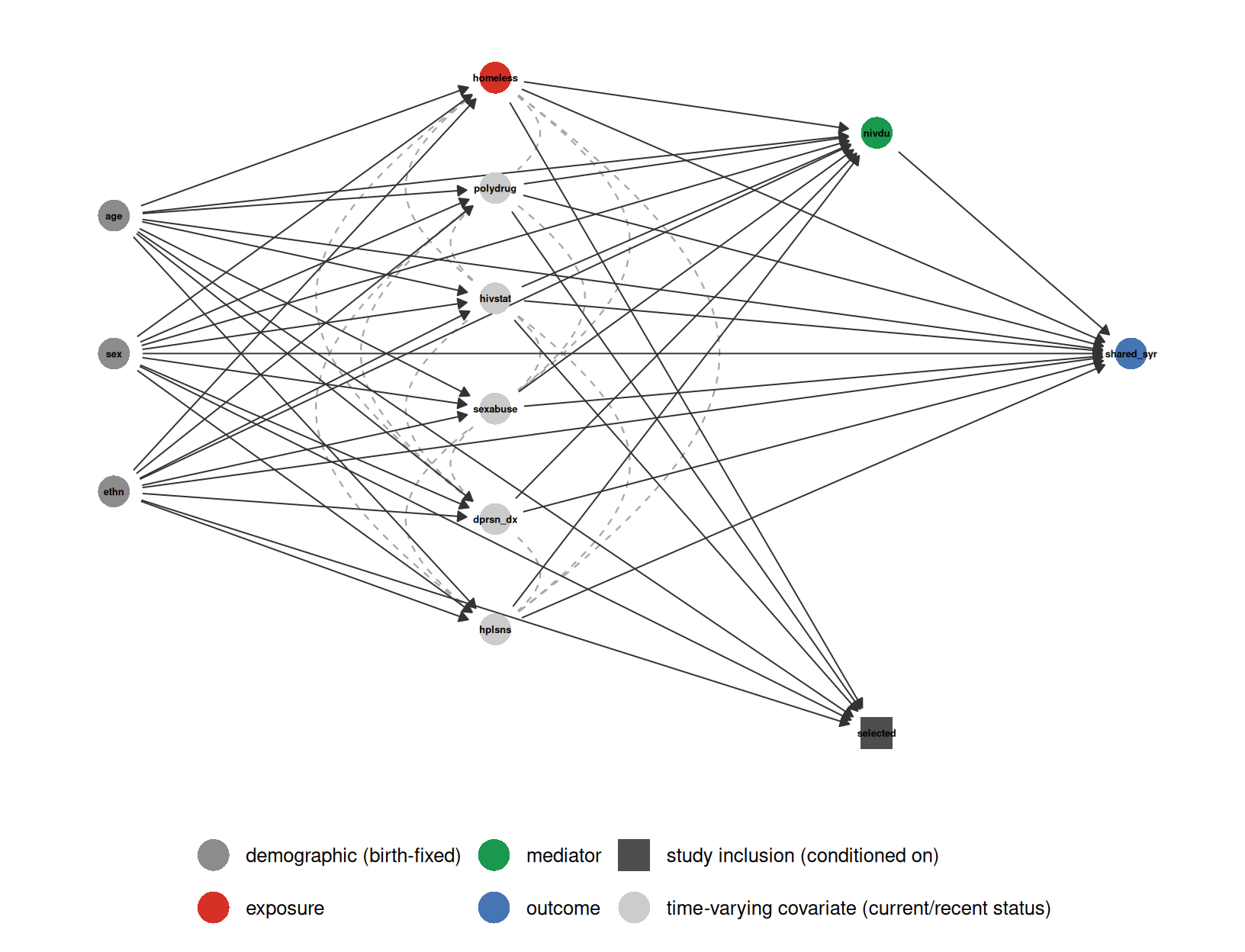
Figure 1: Hypothesized causal structure for the needle-sharing example, drawn for a cross-sectional study. The exposure of interest is homelessness (homeless, red) and the outcome is the count of shared syringes (shared_syr, blue). Injection frequency (nivdu, green) is the one genuine mediator: sharing a syringe requires injecting. Demographic variables (age, sex, ethn, darker grey) are fixed at (or determined by) birth, so they sit upstream of every other variable, with arrows into the time-varying covariates, injection frequency, and the outcome. Because every other covariate is measured at the same single interview, we cannot order the time-varying covariates (lighter grey) causally among themselves; their mutual associations — from shared, unobserved earlier circumstances — are drawn as dashed, non-directional edges. Each time-varying covariate may still affect injection frequency and the 30-day outcome, shown as solid arrows into nivdu and shared_syr. The study-inclusion indicator (selected, square) is conditioned on by design; because several covariates influence who is sampled, conditioning on it can induce associations among them (selection bias).

We treat homelessness as the exposure of interest and ask how it affects the number of shared syringes — following Vittinghoff et al. (2012, sec. 8.3.1), who model this outcome on homeless.

Injection frequency nivdu is a mediator: a shared syringe is necessarily one of the injections, so homelessness can raise sharing partly by raising how often a person injects. Because nivdu lies on the causal path from homeless to shared_syr, we do not adjust for it (neither as a covariate nor as an offset); doing so would block that path and estimate only a partial effect. We want the total effect of homelessness on needle-sharing.

Because the study is cross-sectional, the remaining covariates are measured at the same interview as the exposure, so we cannot order them causally relative to homeless or to one another. We draw their mutual associations as non-directional (bidirected) edges and adjust for the measured covariates to control the confounding they carry. A single fitted coefficient is therefore an adjusted association, not an isolated causal effect.

Conditioning on study inclusion (selected) is unavoidable — we only observe people who were sampled — but because several covariates influence who is sampled, it can induce selection bias that no covariate adjustment removes.

needles

Table 3: Needle-sharing data

---

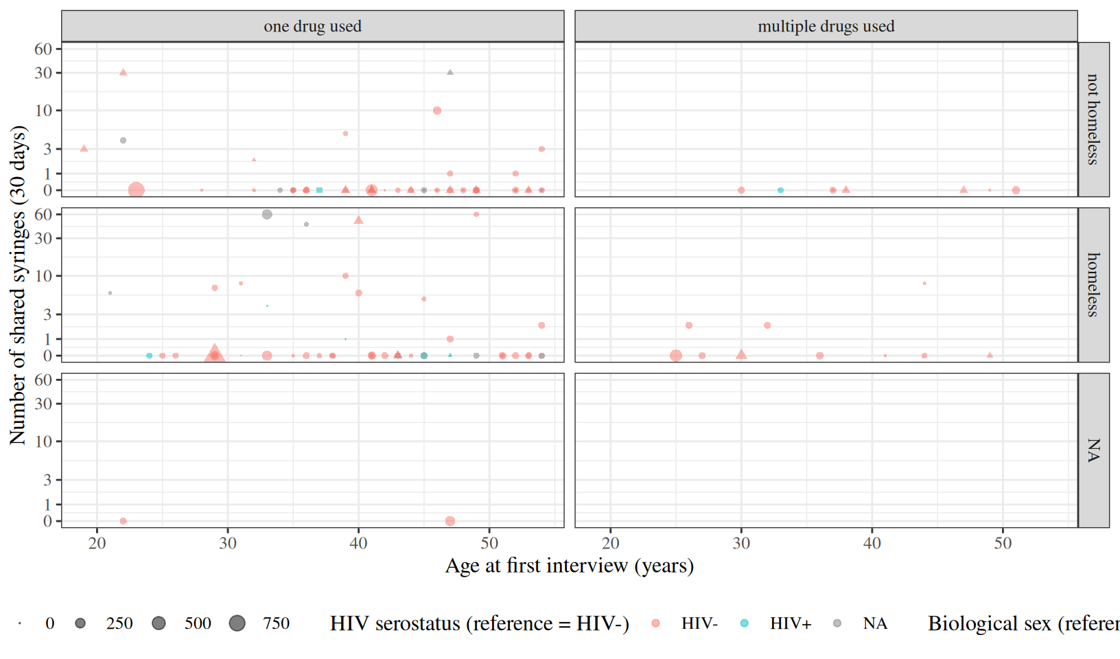
Figure 2 plots the shared-syringe counts against age, split by the covariate subgroups (point size shows injection frequency).

library(ggplot2)

needles |>
  ggplot() +
  aes(
    x = age,
    y = shared_syr,
    shape = sex,
    col = hivstat
  ) +
  geom_point(aes(size = nivdu), alpha = .5) +
  scale_size_area(max_size = 4) +
  scale_y_continuous(
    transform = "pseudo_log",
    breaks = c(0, 1, 3, 10, 30, 60)
  ) +
  facet_grid(cols = vars(polydrug), rows = vars(homeless)) +
  labs(y = "Number of shared syringes (30 days)") +
  theme(legend.position = "bottom")

Figure 2: Needle-sharing counts by age

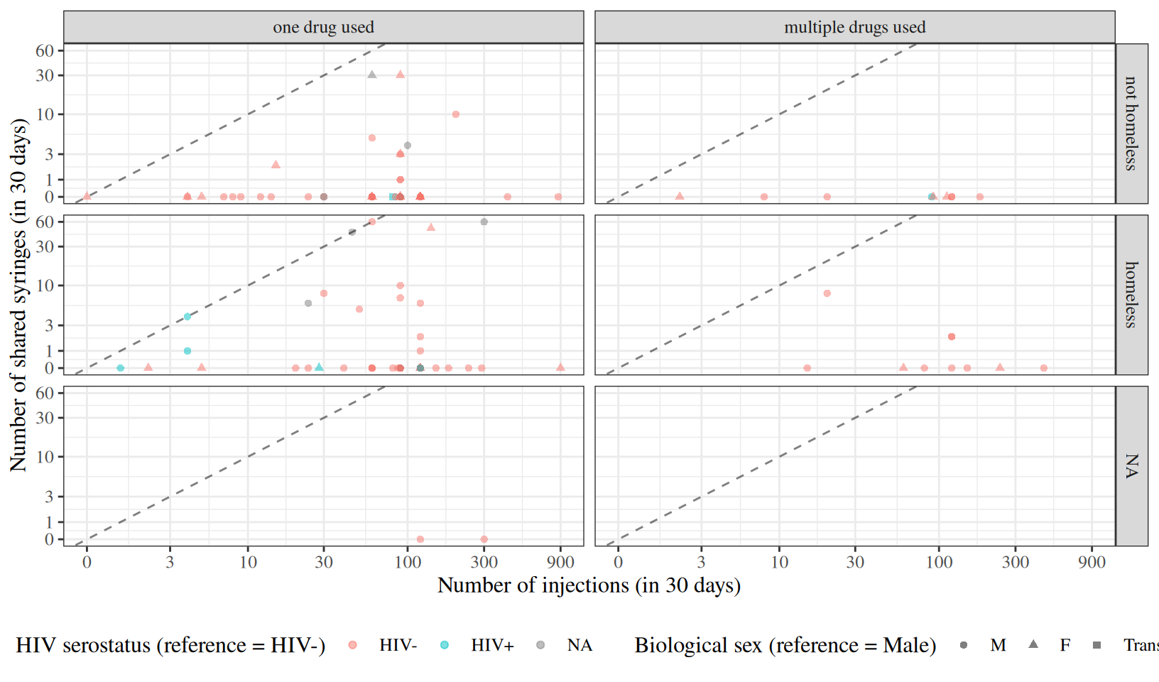
Figure 3 shows the underlying counts: the number of shared syringes against the number of injections, with a dashed \(y = x\) line marking the ceiling where every injection involves a shared syringe.

library(ggplot2)

needles |>
  ggplot() +
  aes(
    x = nivdu,
    y = shared_syr,
    shape = sex,
    col = hivstat
  ) +
  geom_point(alpha = .5) +
  geom_abline(slope = 1, intercept = 0, linetype = "dashed", alpha = .5) +
  # both axes are counts, so pseudo-log both: a shared transform keeps the
  # y = x reference line straight (data diagonal -> panel diagonal)
  scale_x_continuous(
    transform = "pseudo_log",
    breaks = c(0, 3, 10, 30, 100, 300, 900)
  ) +
  scale_y_continuous(
    transform = "pseudo_log",
    breaks = c(0, 1, 3, 10, 30, 60)
  ) +
  facet_grid(cols = vars(polydrug), rows = vars(homeless)) +
  labs(
    x = "Number of injections (in 30 days)",
    y = "Number of shared syringes (in 30 days)"
  ) +
  theme(legend.position = "bottom")

Figure 3: Number of shared syringes versus number of injections (raw counts, 30-day window). The dashed line marks \(y = x\) (every injection involves a shared syringe).

---

3.2 Covariate counts

Table 4: Counts in needles by sex, housing status, and multiple drug use

needles |>
  dplyr::select(sex, homeless, polydrug) |>
  summary()
#>     sex             homeless                 polydrug  
#>  M    :97   not homeless:63   one drug used      :109  
#>  F    :30   homeless    :61   multiple drugs used: 19  
#>  Trans: 1   NAs         : 4

---

There’s only one individual with sex = Trans, which unfortunately isn’t enough data to analyze. We will remove that individual:

needles <- needles |> filter(sex != "Trans")

---

3.3 Model

Following Vittinghoff et al. (2012, sec. 8.3.1), we take homelessness as the exposure of interest and ask how it affects the count of shared syringes, using a Poisson regression (log link) rather than modeling a rate. The remaining covariates enter as adjustments for confounding (Figure 1): because the study is cross-sectional, they are mutually associated with homelessness through shared, unobserved earlier circumstances, which we cannot resolve into a causal order.

Exercise 4 A Poisson rate model would add offset(log(nivdu)), forcing the expected count to be proportional to injection frequency (the coefficient of log(nivdu) fixed at exactly 1). Why not use nivdu as an offset here?

SolutionSolution

Solution 4. We avoid an offset here for two reasons:

• nivdu is a mediator, not an exposure window. An offset is appropriate when its variable is a known denominator — person-time or population at risk — that is external to the causal question. Injection frequency is instead on the causal path from homelessness to sharing (Figure 1): being homeless can raise sharing partly by raising how often a person injects. Conditioning on it (whether as an offset or as a covariate) would block that path and estimate only a partial effect. We want the total effect of homelessness on needle-sharing.
• It imposes an untested proportionality assumption. Fixing the log(nivdu) coefficient at 1 assumes sharing scales one-for-one with injecting, which the data need not support.

Vittinghoff’s analysis uses neither an offset nor nivdu as a covariate.

TipRule of thumb

An offset’s exposure is usually something fixed by the study design — person-time of follow-up, population at risk, area surveyed, number of trials — a known denominator that is exogenous to the question (not caused by the predictors of interest). When the candidate denominator is instead something the participants did, and the predictors also influence it (here, how often they inject), it is a mediator rather than an exposure window, and we model the count directly instead of dividing by it.

We adjust for the measured covariates to control the confounding they carry in Figure 1 — demographic (age, sex, ethn), social (polydrug), serostatus (hivstat), and trauma/mental-health (sexabuse, hopelessness score hplsns) — using main effects only. We exclude the mediator nivdu (discussed in Exercise 4) and the depression indicator dprsn_dx, whose 1/5 coding is undocumented in the source data and so cannot be interpreted.

glm1 <- glm(
  formula = shared_syr ~ homeless +
    age + sex + ethn + polydrug + hivstat + sexabuse + hplsns,
  family = stats::poisson,
  data = needles
)
library(equatiomatic)
equatiomatic::extract_eq(glm1)

\[ \log ({ E( \operatorname{shared_syr} ) }) = \alpha + \beta_{1}(\operatorname{homeless}) + \beta_{2}(\operatorname{age}) + \beta_{3}(\operatorname{sex}_{\operatorname{F}}) + \beta_{4}(\operatorname{ethn}_{\operatorname{AA}}) + \beta_{5}(\operatorname{ethn}_{\operatorname{Hispanic}}) + \beta_{6}(\operatorname{ethn}_{\operatorname{Other}}) + \beta_{7}(\operatorname{polydrug}) + \beta_{8}(\operatorname{hivstat}_{\operatorname{HIV+}}) + \beta_{9}(\operatorname{sex}_{\operatorname{abuseyes}} \times \operatorname{sexabuse}_{\operatorname{yes}}) + \beta_{10}(\operatorname{hplsns}) \]

---

library(parameters)
glm1 |>
  parameters(exponentiate = TRUE) |>
  print_md()

Table 5: Poisson count model for needle-sharing data

Parameter	IRR	SE	95% CI	z	p
(Intercept)	3.69	1.35	(1.78, 7.46)	3.58	< .001
homeless (homeless)	6.04	1.01	(4.38, 8.45)	10.73	< .001
age	0.96	8.79e-03	(0.94, 0.97)	-4.75	< .001
sex (F)	2.42	0.36	(1.81, 3.23)	5.97	< .001
ethn (AA)	2.59	0.48	(1.80, 3.74)	5.13	< .001
ethn (Hispanic)	1.78	0.57	(0.91, 3.20)	1.81	0.070
ethn (Other)	1.04	0.41	(0.44, 2.08)	0.09	0.927
polydrug (multiple drugs used)	0.19	0.06	(0.10, 0.33)	-5.48	< .001
hivstat (HIV+)	0.11	0.05	(0.04, 0.25)	-4.72	< .001
sexabuse (yes)	0.23	0.07	(0.12, 0.40)	-4.71	< .001
hplsns	0.97	0.01	(0.94, 1.00)	-2.21	0.027

---

library(ggplot2)

# Predicted expected counts across age for the two homelessness groups,
# holding the other covariates at their reference levels (hplsns at its
# median). The model has no offset, so predict(type = "response") returns
# the expected number of shared syringes directly.
ref_lvl <- function(v) levels(glm1$model[[v]])[1]
pred_grid <- expand.grid(
  age = seq(min(glm1$model$age), max(glm1$model$age), length.out = 100),
  homeless = levels(glm1$model$homeless),
  sex = ref_lvl("sex"),
  ethn = ref_lvl("ethn"),
  polydrug = ref_lvl("polydrug"),
  hivstat = ref_lvl("hivstat"),
  sexabuse = ref_lvl("sexabuse"),
  hplsns = median(glm1$model$hplsns)
)
pred_grid$shared_syr <- predict(glm1, newdata = pred_grid, type = "response")

ggplot(glm1$model) +
  aes(x = age, y = shared_syr, colour = homeless) +
  geom_point(alpha = 0.4) +
  geom_line(data = pred_grid, linewidth = 1) +
  scale_y_continuous(
    transform = "pseudo_log",
    breaks = c(0, 1, 3, 10, 30, 60)
  ) +
  labs(
    y = "Number of shared syringes (30 days)",
    colour = "Housing status"
  ) +
  theme_bw() +
  theme(legend.position = "bottom")

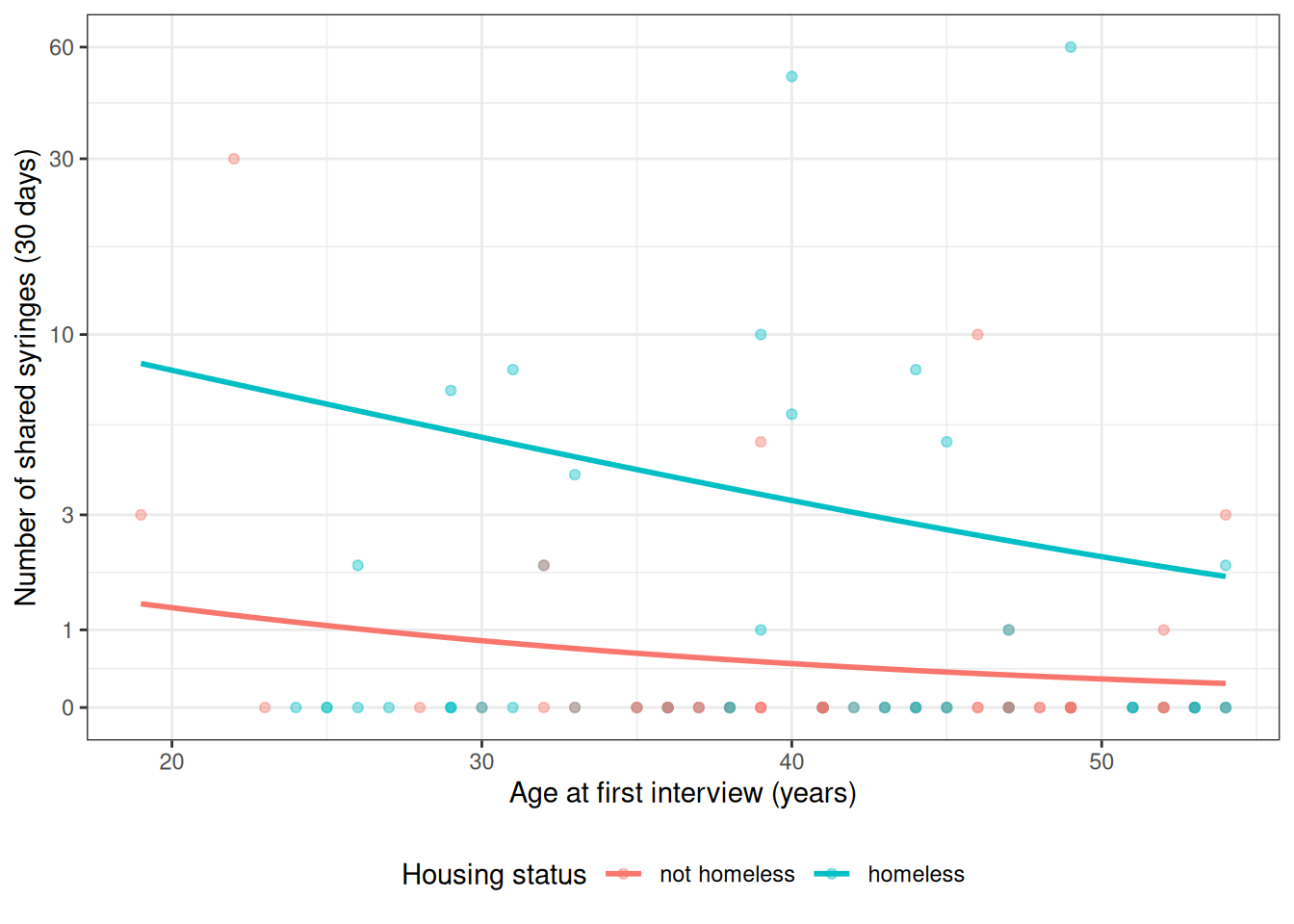
Figure 4: Fitted Poisson model: expected sharing by age and housing status

3.4 Interpreting the coefficients

For a Poisson model with a log link, exponentiating a coefficient turns it into a ratio of expected counts (an incidence rate ratio, IRR, in Vittinghoff et al. (2012)’s terminology): \(\operatorname{exp}\mathopen{}\left\{\beta_j\right\}\mathclose{}\) is the multiplicative change in the expected number of shared syringes per one-unit increase in \(x_j\), holding the other covariates fixed. Our focal estimate is the IRR for homelessness; the remaining coefficients are adjustments for confounding, not effects of separate interest. Because we do not condition on the mediator nivdu, the homelessness IRR is a total effect. The fitted ratios are reported in Table 5.

irr <- exp(coef(glm1))

Baseline (intercept). \(\operatorname{exp}\mathopen{}\left\{\hat\beta_0\right\}\mathclose{} = 3.69\) is the expected count of shared syringes for the reference participant (male, not homeless, White, one drug used, HIV-negative, no sexual-abuse history, hopelessness score 0), extrapolated to age 0. Age 0 is outside the data, so the intercept is a mathematical anchor rather than a directly interpretable quantity.

Age. \(\operatorname{exp}\mathopen{}\left\{\hat\beta_{\text{age}}\right\}\mathclose{} = 0.957\) per year: essentially no association between age and the expected count.

Sex. \(\operatorname{exp}\mathopen{}\left\{\hat\beta_{\text{sexF}}\right\}\mathclose{} = 2.42\): women’s expected count of shared syringes is about 2.42 times men’s, adjusting for the other covariates.

Homelessness (the focal exposure). \(\operatorname{exp}\mathopen{}\left\{\hat\beta_{\text{homeless}}\right\}\mathclose{} = 6.04\): homeless participants share syringes about 6.04 times as often as the non-homeless, adjusting for the other covariates. Vittinghoff et al. (2012, sec. 8.3.1) reports an unadjusted IRR of about 3.3 for homelessness in a single-predictor model; adjusting for the confounder-proxies here moves the estimate to about 6.

Multiple-drug use. \(\operatorname{exp}\mathopen{}\left\{\hat\beta_{\text{polydrug}}\right\}\mathclose{} = 0.19\): multiple-drug users have a lower expected count than single-drug users, though only 19 participants used multiple drugs, so this estimate is imprecise.

HIV serostatus. \(\operatorname{exp}\mathopen{}\left\{\hat\beta_{\text{hivstatHIV+}}\right\}\mathclose{} = 0.11\): HIV-positive participants have a lower expected count of shared syringes than HIV-negative participants, adjusting for the other covariates. Only 8 participants are HIV+ in this sample, so this estimate is imprecise.

Ethnicity. The ethn coefficients compare each retained group to the White reference (small groups were lumped into “Other”); they adjust for any confounding of the homelessness effect by ethnicity but are not of separate interest.

Sexual-abuse history. \(\operatorname{exp}\mathopen{}\left\{\hat\beta_{\text{sexabuse}}\right\}\mathclose{} = 0.23\): participants with a history of sexual abuse share syringes about 0.23 times as often as those without, adjusting for the other covariates.

Hopelessness. \(\operatorname{exp}\mathopen{}\left\{\hat\beta_{\text{hplsns}}\right\}\mathclose{} = 0.97\) per point: each one-point increase in the hopelessness score multiplies the expected count by 0.97, adjusting for the other covariates.

WarningOverdispersion caveat

These data are highly overdispersed — the variance far exceeds the mean — so the model-based Poisson standard errors are too small. Vittinghoff et al. (2012, sec. 8.3.1) recommends robust standard errors or a negative-binomial model for this example.

4 Inference for count regression models

4.0.1 Confidence intervals for regression coefficients and rate ratios

A Wald 95% confidence interval for a single coefficient \(\beta_j\) is:

\[ \beta_j \in \mathopen{}\left[\hat{\beta}_j \pm z_{1 - \frac{\alpha}{2}}\cdot \mathop{\widehat{\operatorname{se}}}\nolimits\mathopen{}\left(\hat{\beta}_j\right)\mathclose{}\right]\mathclose{} \]

where \(z_{1-\alpha/2} \approx 1.96\) for \(\alpha = 0.05\).

Because the log-rate scale is related to the rate scale by exponentiation, we obtain a confidence interval for the rate ratio \(\operatorname{exp}\mathopen{}\left\{\beta_j\right\}\mathclose{}\) by exponentiating both endpoints:

\[ \operatorname{exp}\mathopen{}\left\{\beta_j\right\}\mathclose{} \in \mathopen{}\left[ \operatorname{exp}\mathopen{}\left\{\hat{\beta}_j - z_{1 - \frac{\alpha}{2}}\cdot \mathop{\widehat{\operatorname{se}}}\nolimits\mathopen{}\left(\hat{\beta}_j\right)\mathclose{}\right\}\mathclose{},\; \operatorname{exp}\mathopen{}\left\{\hat{\beta}_j + z_{1 - \frac{\alpha}{2}}\cdot \mathop{\widehat{\operatorname{se}}}\nolimits\mathopen{}\left(\hat{\beta}_j\right)\mathclose{}\right\}\mathclose{} \right]\mathclose{} \]

4.0.2 Hypothesis tests for regression coefficients

To test \(H_0: \beta_j = \beta_{j,0}\) against a one- or two-sided alternative, compute the Wald \(z\)-statistic:

\[ z = \frac{\hat{\beta}_j - \beta_{j,0}}{\mathop{\widehat{\operatorname{se}}}\nolimits\mathopen{}\left(\hat{\beta}_j\right)\mathclose{}} \]

and compare \(z\) (one-sided) or \(|z|\) (two-sided) to the tails of the standard Gaussian distribution. The most common null hypothesis is \(H_0: \beta_j = 0\), i.e., that covariate \(j\) has no association with the outcome rate.

4.0.3 Comparing nested models

To compare a smaller model \(M_0\) (with \(p_0\) parameters) to a larger model \(M_1\) (with \(p_1 > p_0\) parameters), use the likelihood ratio test statistic:

\[ G^2 = 2\mathopen{}\left[\hat{\ell}_1 - \hat{\ell}_0\right]\mathclose{} \]

where \(\hat{\ell}_1\) and \(\hat{\ell}_0\) are the maximized log-likelihoods of \(M_1\) and \(M_0\) respectively.

Under \(H_0\) that the additional \(p_1 - p_0\) parameters are all zero, \(G^2 \ \dot{\sim} \ \chi^2_{p_1 - p_0}\).

See Dobson and Barnett (2018, chap. 9) and Vittinghoff et al. (2012, sec. 8.1) for details.

5 Prediction

\[ \begin{aligned} \hat{y} &\stackrel{\text{def}}{=}\mathop{\hat{\operatorname{E}}}\nolimits\mathopen{}\left[Y \mid \tilde{X}= \tilde{x}, T = t\right]\mathclose{} \\ &\quad \text{(definition of estimated conditional expectation)} \\ &= \hat{\mu}(\tilde{x}, t) \\ &\quad \text{(estimated mean count function)} \\ &= \hat{\lambda}(\tilde{x}) \cdot t \\ &\quad \text{(substituting the estimated rate relation)} \\ &= \operatorname{exp}\mathopen{}\left\{\hat{\eta}(\tilde{x})\right\}\mathclose{} \cdot t \\ &\quad \text{(substituting the inverse link function)} \\ &= \operatorname{exp}\mathopen{}\left\{\hat{\beta}_0 + \hat{\beta}_1 x_1 + \dots + \hat{\beta}_p x_p\right\}\mathclose{} \cdot t \\ &\quad \text{(substituting estimated linear predictor } \hat{\eta}(\tilde{x})\text{)} \end{aligned} \]

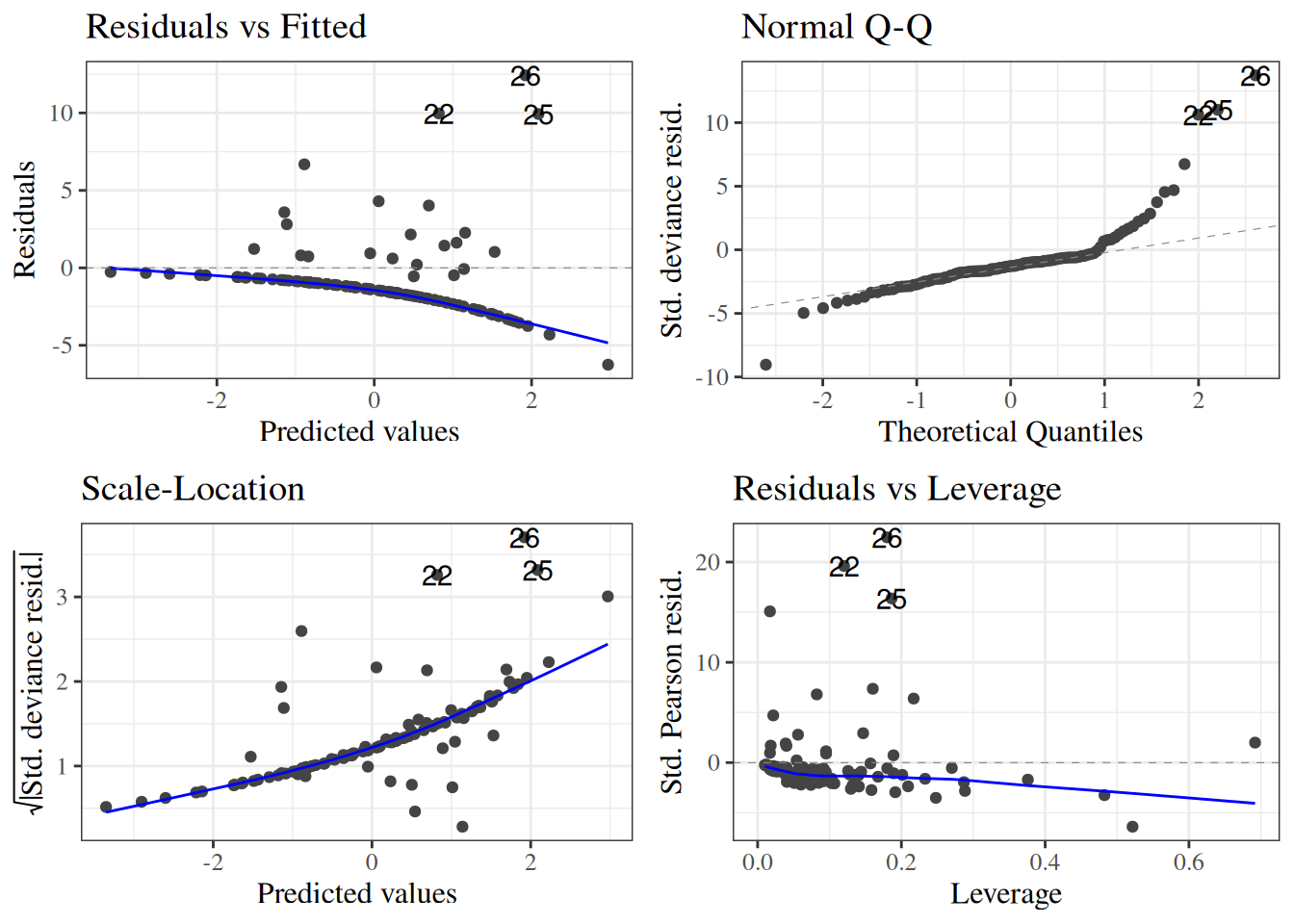
6 Diagnostics

6.0.1 Residuals

Observation residuals

\[e_i \stackrel{\text{def}}{=}y_i - \hat{y}_i\]

Pearson residuals

\[r_i \stackrel{\text{def}}{=}\frac{e_i}{\mathop{\widehat{\operatorname{se}}}\nolimits\mathopen{}\left(e_i\right)\mathclose{}} \approx \frac{e_i}{\sqrt{\hat{y}_i}}\]

Standardized Pearson residuals

\[r_{p,i} \stackrel{\text{def}}{=}\frac{r_i}{\sqrt{1-h_i}}\] where \(h_i\) is the leverage of observation \(i\): the \(i\)-th diagonal element of the weighted hat matrix. That definition is stated for a logistic model, so it uses binomial weights; for Poisson regression the corresponding weight is \(\hat{\mu}_i\). That definition also indexes covariate patterns, which here we take to be the individual observations.

Deviance residuals

\[ d_i \stackrel{\text{def}}{=}\operatorname{sign}(y_i - \hat{y}_i) \sqrt{2\mathopen{}\left[\ell_{\text{full}}(y_i) - \ell(\hat{\tilde{\beta}}; y_i)\right]\mathclose{}} \]

Note

\[ \operatorname{sign}(x) \stackrel{\text{def}}{=} \begin{cases} \frac{x}{|x|} & x \neq 0\\ 0 & x = 0 \end{cases} \] In other words:

• \(\operatorname{sign}(x) = -1\) if \(x < 0\)
• \(\operatorname{sign}(x) = 0\) if \(x = 0\)
• \(\operatorname{sign}(x) = 1\) if \(x > 0\)

---

library(ggfortify)
autoplot(glm1)

Table 6: Diagnostics for Poisson model

7 Zero-inflation

7.0.1 Models for zero-inflated counts

We assume a latent (unobserved) binary variable, \(Z\), which we model using logistic regression:

\[ \begin{aligned} \pi(\tilde{x}) &\stackrel{\text{def}}{=}\operatorname{P}(Z=1 \mid \tilde{X}=\tilde{x})\\ &= \operatorname{expit}(\gamma_0 + \gamma_1 x_1 + \dots + \gamma_p x_p) \end{aligned} \]

The model makes \(Z\) depend on the covariates alone, not on the exposure magnitude \(T\), so \(\operatorname{P}(Z=1 \mid \tilde{X}=\tilde{x}, T=t) = \pi(\tilde{x})\) for every \(t\) — that is, \(Z \perp\!\!\!\perp T \mid \tilde{X}\).

According to this model, if \(Z=1\), then \(Y\) will always be zero, regardless of \(\tilde{X}\) and \(T\):

\[\operatorname{P}(Y=0 \mid Z=1, \tilde{X}=\tilde{x}, T=t) = 1\]

Otherwise (if \(Z=0\)), \(Y\) follows a Poisson distribution, conditional on \(\tilde{X}\) and \(T\), as in a standard Poisson regression model.

Throughout this section, abbreviate \(\pi \stackrel{\text{def}}{=}\pi(\tilde{x})\) and \(\mu_0 \stackrel{\text{def}}{=}\operatorname{E}[Y \mid Z=0, \tilde{X}=\tilde{x}, T=t]\). Since the \(Z=0\) arm is an ordinary Poisson regression model, \(\mu_0 = t \operatorname{exp}\mathopen{}\left\{\eta(\tilde{x})\right\}\mathclose{}\) by Equation 1, which is strictly positive whenever \(t > 0\).

Even though we never observe \(Z\), we can estimate the parameters \(\gamma_0, \dots, \gamma_p\) via maximum likelihood:

\[ \begin{aligned} \operatorname{P}(Y=y \mid \tilde{X}=\tilde{x}, T=t) &= \operatorname{P}(Y=y, Z=1 \mid \tilde{X}=\tilde{x}, T=t) \\ &\phantom{={}} + \operatorname{P}(Y=y, Z=0 \mid \tilde{X}=\tilde{x}, T=t) \\ &\quad \text{(by Law of Total Probability)} \end{aligned} \]

where \[ \begin{aligned} \operatorname{P}(Y=y, Z=z \mid \tilde{X}=\tilde{x}, T=t) &= \operatorname{P}(Y=y \mid Z=z, \tilde{X}=\tilde{x}, T=t) \operatorname{P}(Z=z \mid \tilde{X}=\tilde{x}) \\ &\quad \text{(with } Z \perp\!\!\!\perp T \mid \tilde{X}\text{)} \end{aligned} \]

Exercise 5 Expand \(\operatorname{P}(Y=0 \mid \tilde{X}=\tilde{x}, T=t)\), \(\operatorname{P}(Y=1 \mid \tilde{X}=\tilde{x}, T=t)\), and \(\operatorname{P}(Y=y \mid \tilde{X}=\tilde{x}, T=t)\) into expressions involving \(\pi\) and \(\mu_0\).

SolutionSolution

Solution. \(\operatorname{P}(Y=0)\): \(Y=0\) occurs either because \(Z=1\) (always zero) or because \(Z=0\) and the Poisson draw equals 0:

\[ \begin{aligned} \operatorname{P}(Y=0 \mid \tilde{X}=\tilde{x}, T=t) &= \pi \, \operatorname{P}(Y=0 \mid Z=1, \tilde{X}=\tilde{x}, T=t) \\ &\phantom{={}} + (1-\pi) \, \operatorname{P}(Y=0 \mid Z=0, \tilde{X}=\tilde{x}, T=t) \\ &\quad \text{(by Law of Total Probability; } Z \perp\!\!\!\perp T \mid \tilde{X}\text{)} \\ &= \pi \cdot 1 + (1-\pi) \operatorname{exp}\mathopen{}\left\{-\mu_0\right\}\mathclose{} \\ &\quad \text{(substituting the two conditional PMFs)} \\ &= \pi + (1-\pi) \operatorname{exp}\mathopen{}\left\{-\mu_0\right\}\mathclose{} \\ &\quad \text{(simplifying arithmetic)} \end{aligned} \]

\(\operatorname{P}(Y=1)\): \(Z=1\) can never produce \(Y=1\), so:

\[ \begin{aligned} \operatorname{P}(Y=1 \mid \tilde{X}=\tilde{x}, T=t) &= \pi \, \operatorname{P}(Y=1 \mid Z=1, \tilde{X}=\tilde{x}, T=t) \\ &\phantom{={}} + (1-\pi) \, \operatorname{P}(Y=1 \mid Z=0, \tilde{X}=\tilde{x}, T=t) \\ &\quad \text{(by Law of Total Probability; } Z \perp\!\!\!\perp T \mid \tilde{X}\text{)} \\ &= \pi \cdot 0 + (1-\pi) \mu_0 \operatorname{exp}\mathopen{}\left\{-\mu_0\right\}\mathclose{} \\ &\quad \text{(since } \operatorname{P}(Y=1 \mid Z=1, \tilde{X}=\tilde{x}, T=t)=0\text{)} \\ &= (1-\pi) \mu_0 \operatorname{exp}\mathopen{}\left\{-\mu_0\right\}\mathclose{} \\ &\quad \text{(simplifying arithmetic)} \end{aligned} \]

\(\operatorname{P}(Y=y)\) for \(y \geq 1\): Identical reasoning gives:

\[ \begin{aligned} \operatorname{P}(Y=y \mid \tilde{X}=\tilde{x}, T=t) &= \pi \, \operatorname{P}(Y=y \mid Z=1, \tilde{X}=\tilde{x}, T=t) \\ &\phantom{={}} + (1-\pi) \, \operatorname{P}(Y=y \mid Z=0, \tilde{X}=\tilde{x}, T=t) \\ &\quad \text{(by Law of Total Probability; } Z \perp\!\!\!\perp T \mid \tilde{X}\text{)} \\ &= \pi \cdot 0 + (1-\pi) \frac{\mu_0^y \operatorname{exp}\mathopen{}\left\{-\mu_0\right\}\mathclose{}}{y!} \\ &\quad \text{(since } \operatorname{P}(Y=y \mid Z=1, \tilde{X}=\tilde{x}, T=t)=0 \text{ for } y \geq 1\text{)} \\ &= (1-\pi) \frac{\mu_0^y \operatorname{exp}\mathopen{}\left\{-\mu_0\right\}\mathclose{}}{y!} \\ &\quad \text{(simplifying arithmetic)} \end{aligned} \]

Exercise 6 Derive the expected value and variance of \(Y\), conditional on \(\tilde{X}=\tilde{x}\) and \(T=t\), as functions of \(\pi\) and \(\mu_0\).

SolutionSolution

Solution. Expected value. By the Law of Total Expectation (conditioning on \(Z\), within the subpopulation \(\{\tilde{X}=\tilde{x}, T=t\}\)):

\[ \begin{aligned} \operatorname{E}[Y \mid \tilde{X}=\tilde{x}, T=t] &= \pi \, \operatorname{E}[Y \mid Z=1, \tilde{X}=\tilde{x}, T=t] \\ &\phantom{={}} + (1-\pi) \, \operatorname{E}[Y \mid Z=0, \tilde{X}=\tilde{x}, T=t] \\ &\quad \text{(by Law of Total Expectation; } Z \perp\!\!\!\perp T \mid \tilde{X}\text{)} \\ &= 0 \cdot \pi + \mu_0 (1-\pi) \\ &\quad \text{(substituting the conditional means)} \\ &= (1-\pi) \mu_0 \\ &\quad \text{(simplifying arithmetic)} \end{aligned} \]

The substitution \(\operatorname{E}[Y \mid Z=0, \tilde{X}=\tilde{x}, T=t] = \mu_0\) follows immediately from the definition of \(\mu_0\).

Variance. Within this derivation, write \(\operatorname{E}[\,\cdot \mid Z]\) and \(\operatorname{Var}\mathopen{}\left(\cdot \mid Z\right)\mathclose{}\) for the moments conditional on \(Z\) and on \(\tilde{X}=\tilde{x}, T=t\); the outer operators keep their conditioning explicit. By the Law of Total Variance:

\[ \begin{aligned} \operatorname{Var}\mathopen{}\left(Y \mid \tilde{X}=\tilde{x}, T=t\right)\mathclose{} &= \operatorname{E}\mathopen{}\left[\operatorname{Var}\mathopen{}\left(Y \mid Z\right)\mathclose{} \mid \tilde{X}=\tilde{x}, T=t\right]\mathclose{} \\ &\phantom{={}} + \operatorname{Var}\mathopen{}\left(\operatorname{E}[Y \mid Z] \mid \tilde{X}=\tilde{x}, T=t\right)\mathclose{} \\ &\quad \text{(by Law of Total Variance)} \end{aligned} \]

For the expected conditional variance term, note that

\[\operatorname{Var}\mathopen{}\left(Y \mid Z=1\right)\mathclose{} = 0 \quad\text{and}\quad \operatorname{Var}\mathopen{}\left(Y \mid Z=0\right)\mathclose{} = \mu_0\]

since the \(Z=0\) arm is Poisson, so:

\[ \begin{aligned} \operatorname{E}\mathopen{}\left[\operatorname{Var}\mathopen{}\left(Y \mid Z\right)\mathclose{} \mid \tilde{X}=\tilde{x}, T=t\right]\mathclose{} &= \pi \, \operatorname{Var}\mathopen{}\left(Y \mid Z=1\right)\mathclose{} + (1-\pi) \, \operatorname{Var}\mathopen{}\left(Y \mid Z=0\right)\mathclose{} \\ &\quad \text{(expectation over } Z\text{; } Z \perp\!\!\!\perp T \mid \tilde{X}\text{)} \\ &= 0 \cdot \pi + \mu_0 (1-\pi) \\ &\quad \text{(substituting the conditional variances)} \\ &= (1-\pi)\mu_0 \\ &\quad \text{(simplifying arithmetic)} \end{aligned} \]

For the variance of conditional expectation term, \(\operatorname{E}[Y \mid Z]\) takes value 0 (with probability \(\pi\)) or \(\mu_0\) (with probability \(1-\pi\)), so:

\[ \begin{aligned} \operatorname{Var}\mathopen{}\left(\operatorname{E}[Y \mid Z] \mid \tilde{X}=\tilde{x}, T=t\right)\mathclose{} &= \pi \mathopen{}\left(0 - (1-\pi)\mu_0\right)\mathclose{}^2 + (1-\pi) \mathopen{}\left(\mu_0 - (1-\pi)\mu_0\right)\mathclose{}^2 \\ &\quad \text{(variance over } Z\text{; } Z \perp\!\!\!\perp T \mid \tilde{X}\text{)} \\ &= \pi(1-\pi)^2 \mu_0^2 + (1-\pi)\pi^2 \mu_0^2 \\ &\quad \text{(expanding squared terms)} \\ &= \pi(1-\pi)\mu_0^2 \mathopen{}\left[(1-\pi) + \pi\right]\mathclose{} \\ &\quad \text{(factoring)} \\ &= \pi(1-\pi)\mu_0^2 \\ &\quad \text{(since } (1-\pi) + \pi = 1\text{)} \end{aligned} \]

Combining both terms gives:

\[ \begin{aligned} \operatorname{Var}\mathopen{}\left(Y \mid \tilde{X}=\tilde{x}, T=t\right)\mathclose{} &= (1-\pi)\mu_0 + \pi(1-\pi)\mu_0^2 \\ &\quad \text{(summing expected variance and variance of expectation)} \\ &= (1-\pi)\mu_0 \mathopen{}\left(1 + \pi\mu_0\right)\mathclose{} \\ &\quad \text{(factoring out } (1-\pi)\mu_0\text{)} \end{aligned} \]

The logistic model puts \(\pi\) strictly between 0 and 1, since \(\operatorname{expit}\) never attains its limits, and \(\mu_0 = t \operatorname{exp}\mathopen{}\left\{\eta(\tilde{x})\right\}\mathclose{} > 0\) whenever \(t > 0\). Then \(1 + \pi\mu_0 > 1\), so

\[(1-\pi)\mu_0 (1+\pi\mu_0) > (1-\pi)\mu_0 = \operatorname{E}[Y \mid \tilde{X}=\tilde{x}, T=t]\]

and a zero-inflated count model is overdispersed relative to a Poisson model with the same mean, at every covariate pattern with positive exposure.

8 Over-dispersion

---

The Poisson distribution model forces the conditional variance to equal the conditional mean (\(\operatorname{Var}\mathopen{}\left(Y \mid \tilde{X}=\tilde{x}, T=t\right)\mathclose{} = \operatorname{E}[Y \mid \tilde{X}=\tilde{x}, T=t]\)). In practice, observational count data frequently exhibit variance substantially larger than the mean (or occasionally smaller, termed underdispersion).

Definition 1 (Overdispersion) Write \(m_{\operatorname{P}}(\tilde{x}, t)\) and \(v_{\operatorname{P}}(\tilde{x}, t)\) for the conditional mean and variance that a model \(\operatorname{P}(Y=y \mid \tilde{X}=\tilde{x}, T=t)\) specifies; for a Poisson model, \(v_{\operatorname{P}}(\tilde{x}, t) = m_{\operatorname{P}}(\tilde{x}, t) = \mu(\tilde{x}, t)\). Let \(\operatorname{P}\) specify \(Y\)’s conditional mean correctly, so that \(m_{\operatorname{P}}(\tilde{x}, t) = \operatorname{E}[Y \mid \tilde{X}=\tilde{x}, T=t]\) for every \(\tilde{x}\) and \(t\). Then \(Y\) is overdispersed relative to \(\operatorname{P}\) if its conditional variance exceeds the one \(\operatorname{P}\) specifies at some covariate pattern and exposure:

\[\operatorname{Var}\mathopen{}\left(Y \mid \tilde{X}=\tilde{x}, T=t\right)\mathclose{} > v_{\operatorname{P}}(\tilde{x}, t)\]

The same-mean requirement is what makes this a statement about dispersion: without it, any model that simply understates the mean would look overdispersed. In practice we detect overdispersion by comparing the conditional empirical variance in a dataset against \(v_{\hat{\operatorname{P}}}(\tilde{x}, t)\), the variance a fitted model predicts.

In Poisson regression, unmodeled heterogeneity, clustering, and omitted predictors all inflate the conditional variance. Where the mean model remains correct, that inflation is overdispersion in the sense of Definition 1. An omitted predictor may instead — or additionally — misspecify the mean, and to whatever extent it does, the model is failing the correct-mean requirement Definition 1 imposes, which is a different problem requiring a different remedy. When overdispersion is present but ignored, the point estimates \(\hat{\tilde{\beta}}\) remain consistent, but the standard errors produced by standard maximum likelihood estimation are severely underestimated. This underestimation leads to overly narrow confidence intervals and inflated false-positive (type I error) rates during hypothesis testing.

When overdispersion is detected via residual diagnostics (such as the deviance or Pearson \(\chi^2\) statistic, divided by its residual degrees of freedom, substantially exceeding 1), practitioners can address it by incorporating missing predictors, using quasipoisson estimation, or fitting a negative binomial regression model.

c.f. Dobson and Barnett (2018) §3.2.1, 7.7, 9.8; Vittinghoff et al. (2012) §8.1.5; and https://en.wikipedia.org/wiki/Overdispersion.

---

Note

Logistic regression is named after the (inverse) link function. Poisson regression is named after the outcome distribution. This naming convention reflects the strongest (and often most questionable) assumption in each model. In binary data regression, the outcome distribution essentially must be Bernoulli (or Binomial), but the link function could be logit, log, identity, probit, or something more unusual. In count data regression, the outcome distribution could have many different shapes, but the link function will probably end up being log, so that covariates have multiplicative effects on the rate.

---

8.1 Negative binomial models

There are alternatives to the Poisson model when overdispersion is present. Most notably, the negative binomial model.

Diagnostics that reveal overdispersion are telling us that the data violate the standard Poisson assumption

\[\operatorname{Var}\mathopen{}\left(Y \mid \tilde{X}=\tilde{x}, T=t\right)\mathclose{} = \operatorname{E}[Y \mid \tilde{X}=\tilde{x}, T=t]\]

Ignoring that violation leads to artificially narrow standard errors and inflated type I error rates. The negative binomial distribution serves as a natural generalization of the Poisson distribution for count outcomes. It introduces an overdispersion parameter \(\rho\) that allows the conditional variance to exceed the mean (\(\operatorname{Var}\mathopen{}\left(Y \mid \tilde{X}=\tilde{x}, T=t\right)\mathclose{} = \mu(\tilde{x}, t) + \mu(\tilde{x}, t)^2 / \rho\)). We still model \(\mu(\tilde{x}, t) = t \operatorname{exp}\mathopen{}\left\{\eta(\tilde{x})\right\}\mathclose{}\) as before, preserving the rate-ratio interpretation for regression coefficients. Furthermore, negative binomial models can be combined with zero-inflation to account for both structural zeros and variance expansion in count data, with the negative binomial serving as the conditional distribution for the count component.

---

8.1.1 Example: needle-sharing model extensions

To evaluate whether overdispersion and excess zeros distort inference in the needle-sharing dataset, we fit a negative binomial model and compare its coefficient estimates and standard errors against the baseline Poisson model.

library(MASS) # for glm.nb()
glm1_nb <- glm.nb(
  formula = shared_syr ~ homeless +
    age + sex + ethn + polydrug + hivstat + sexabuse + hplsns,
  data = needles
)

equatiomatic::extract_eq(glm1_nb)

\[ \log ({ E( \operatorname{shared_syr} ) }) = \alpha + \beta_{1}(\operatorname{homeless}) + \beta_{2}(\operatorname{age}) + \beta_{3}(\operatorname{sex}_{\operatorname{F}}) + \beta_{4}(\operatorname{ethn}_{\operatorname{AA}}) + \beta_{5}(\operatorname{ethn}_{\operatorname{Hispanic}}) + \beta_{6}(\operatorname{ethn}_{\operatorname{Other}}) + \beta_{7}(\operatorname{polydrug}) + \beta_{8}(\operatorname{hivstat}_{\operatorname{HIV+}}) + \beta_{9}(\operatorname{sex}_{\operatorname{abuseyes}} \times \operatorname{sexabuse}_{\operatorname{yes}}) + \beta_{10}(\operatorname{hplsns}) \]

Table 7: Negative binomial model for needle-sharing data

summary(glm1_nb)
#> 
#> Call:
#> glm.nb(formula = shared_syr ~ homeless + age + sex + ethn + polydrug + 
#>     hivstat + sexabuse + hplsns, data = needles, init.theta = 0.08315440712, 
#>     link = log)
#> 
#> Coefficients:
#>                             Estimate Std. Error z value Pr(>|z|)    
#> (Intercept)                   6.4536     1.8421    3.50  0.00046 ***
#> homelesshomeless              1.1508     0.7366    1.56  0.11820    
#> age                          -0.1485     0.0433   -3.43  0.00059 ***
#> sexF                          0.2198     0.8179    0.27  0.78813    
#> ethnAA                        1.5958     0.8890    1.79  0.07265 .  
#> ethnHispanic                  3.7763     1.5240    2.48  0.01322 *  
#> ethnOther                    -3.2365     2.2663   -1.43  0.15327    
#> polydrugmultiple drugs used  -4.0532     1.0898   -3.72  0.00020 ***
#> hivstatHIV+                  -1.1548     1.3185   -0.88  0.38113    
#> sexabuseyes                  -2.6449     1.0772   -2.46  0.01408 *  
#> hplsns                        0.0948     0.0648    1.46  0.14306    
#> ---
#> Signif. codes:  0 '***' 0.001 '**' 0.01 '*' 0.05 '.' 0.1 ' ' 1
#> 
#> (Dispersion parameter for Negative Binomial(0.0913) family taken to be 1)
#> 
#>     Null deviance: 62.231  on 108  degrees of freedom
#> Residual deviance: 60.031  on  98  degrees of freedom
#>   (18 observations deleted due to missingness)
#> AIC: 267.9
#> 
#> Number of Fisher Scoring iterations: 25
#> 
#> 
#>               Theta:  0.0832 
#>           Std. Err.:  0.0216 
#> Warning while fitting theta: alternation limit reached 
#> 
#>  2 x log-likelihood:  -243.8880

---

Evaluating the estimated parameters across models reveals how accounting for overdispersion affects inference. While the estimated log-rate coefficients remain comparable between the Poisson and negative binomial specifications, the standard errors under the negative binomial model appropriately widen to reflect the excess outcome variability.

tibble(
  Parameter = names(coef(glm1)),
  `Poisson Coef` = coef(glm1),
  `Poisson SE` = summary(glm1)$coefficients[, "Std. Error"],
  `NB Coef` = coef(glm1_nb),
  `NB SE` = summary(glm1_nb)$coefficients[, "Std. Error"]
) |>
  pander::pander()

Table 8: Poisson vs. Negative Binomial regression estimates

Parameter	Poisson Coef	Poisson SE	NB Coef	NB SE
(Intercept)	1.306	0.3649	6.454	1.842
homelesshomeless	1.799	0.1676	1.151	0.7366
age	-0.0436	0.009183	-0.1485	0.04326
sexF	0.8835	0.1479	0.2198	0.8179
ethnAA	0.9525	0.1858	1.596	0.889
ethnHispanic	0.5775	0.3183	3.776	1.524
ethnOther	0.03598	0.3933	-3.236	2.266
polydrugmultiple drugs used	-1.676	0.3062	-4.053	1.09
hivstatHIV+	-2.179	0.4617	-1.155	1.319
sexabuseyes	-1.474	0.3132	-2.645	1.077
hplsns	-0.03147	0.01423	0.09484	0.06476

Zero-inflated models for needle-sharing

Because many participants report zero shared syringes in the past 30 days, we fit a zero-inflated Poisson (ZIP) model to distinguish structural non-sharers from count variability.

library(glmmTMB)
zinf_pois <- glmmTMB(
  family = "poisson",
  data = needles,
  formula = shared_syr ~ homeless +
    age + sex + ethn + polydrug + hivstat + sexabuse + hplsns,
  # the zero-inflation submodel uses the exposure, matching Vittinghoff's
  # `inflate(i.homeless)` (@vittinghoff2e, §8.3.1)
  ziformula = ~ homeless
)

zinf_pois |>
  parameters(exponentiate = TRUE) |>
  print_md()

Table 9: Zero-inflated Poisson model

Fixed Effects

Parameter	IRR	SE	95% CI	z	p
(Intercept)	0.42	0.42	(0.06, 2.94)	-0.87	0.385
homeless (homeless)	4.13	0.90	(2.70, 6.32)	6.54	< .001
age	1.02	0.02	(0.99, 1.06)	1.14	0.256
sex (F)	10.01	3.44	(5.10, 19.63)	6.70	< .001
ethn (AA)	11.21	4.24	(5.35, 23.51)	6.40	< .001
ethn (Hispanic)	0.62	0.25	(0.28, 1.36)	-1.20	0.230
ethn (Other)	1.25	0.64	(0.46, 3.42)	0.43	0.664
polydrug (multiple drugs used)	0.98	0.50	(0.36, 2.68)	-0.03	0.974
hivstat (HIV+)	0.36	0.18	(0.14, 0.97)	-2.02	0.044
sexabuse (yes)	0.09	0.03	(0.05, 0.18)	-6.87	< .001
hplsns	1.05	0.03	(0.99, 1.12)	1.66	0.096

Zero-Inflation

Parameter	Odds Ratio	SE	95% CI	z	p
(Intercept)	4.84	1.92	(2.22, 10.55)	3.97	< .001
homeless (homeless)	0.53	0.27	(0.20, 1.44)	-1.24	0.216

Another R package for zero-inflated models is pscl (Zeileis et al. (2008)).

Zero-inflated negative binomial model

To combine flexible dispersion modeling with zero-inflation, we also fit a zero-inflated negative binomial (ZINB) model.

zinf_nb <- glmmTMB(
  family = nbinom2,
  data = needles,
  formula = shared_syr ~ homeless +
    age + sex + ethn + polydrug + hivstat + sexabuse + hplsns,
  ziformula = ~ homeless
)

zinf_nb |>
  parameters(exponentiate = TRUE) |>
  print_md()

Table 10: Zero-inflated negative binomial model

Fixed Effects

Parameter	IRR	SE	95% CI	z	p
(Intercept)	0.58	2.93	(2.76e-05, 12031.38)	-0.11	0.914
homeless (homeless)	2.66	1.94	(0.64, 11.08)	1.34	0.180
age	1.02	0.10	(0.85, 1.23)	0.26	0.798
sex (F)	8.11	13.94	(0.28, 235.47)	1.22	0.223
ethn (AA)	9.40	12.29	(0.72, 121.95)	1.71	0.087
ethn (Hispanic)	0.90	1.38	(0.04, 18.04)	-0.07	0.945
ethn (Other)	1.46	2.97	(0.03, 77.95)	0.19	0.851
polydrug (multiple drugs used)	0.79	2.02	(5.15e-03, 120.47)	-0.09	0.926
hivstat (HIV+)	0.42	0.52	(0.04, 4.72)	-0.70	0.481
sexabuse (yes)	0.09	0.09	(0.01, 0.65)	-2.40	0.016
hplsns	1.03	0.12	(0.83, 1.29)	0.30	0.767

Zero-Inflation

Parameter	Odds Ratio	SE	95% CI	z	p
(Intercept)	4.70	1.94	(2.09, 10.56)	3.75	< .001
homeless (homeless)	0.49	0.26	(0.17, 1.40)	-1.33	0.182

Dispersion

Parameter	Coefficient	95% CI
(Intercept)	1.49	(0.54, 4.09)

Both zero-inflated models keep the zero-inflation (structural-zero) submodel parsimonious — just the exposure, ziformula = ~ homeless — matching Vittinghoff et al. (2012)’s inflate(i.homeless) [§8.3.1].

A richer zero-inflation submodel is poorly identified here. With the negative binomial in particular, the overdispersion parameter and the zero-inflation component both compete to explain the excess zeros, so adding several covariates to the submodel makes the logistic fit separate: its coefficients diverge and the exponentiated estimates (odds ratios) run off to \(\pm\infty\). Keeping the submodel small avoids that.

8.2 Quasipoisson regression

Another way to handle overdispersion — rather than switching to the negative binomial distributional family — is the quasipoisson approach. It assumes less model structure than the negative binomial does: rather than committing to a complete probability distribution and estimating by maximum likelihood, it assumes only the mean-variance relationship \(\operatorname{Var}\mathopen{}\left(Y \mid \tilde{X}=\tilde{x}, T=t\right)\mathclose{} = \theta \mu(\tilde{x}, t)\), for a dispersion parameter \(\theta\). It pairs that single assumption with a moment-based inference method, estimating \(\theta\) from the Pearson residuals.

While point estimates for regression coefficients \(\hat{\tilde{\beta}}\) remain identical to standard Poisson regression, their estimated standard errors are scaled by \(\sqrt{\hat{\theta}}\). This approach provides valid standard errors and \(p\)-values when overdispersion is multiplicative. That validity comes from the assumed mean-variance relationship itself. A sandwich (robust) variance estimator also uses the residuals, but it does not require the model’s variance function to be correct; it accumulates the squared residuals across observations instead of scaling the variance formula the model supplied. Its validity therefore does not depend on that variance function being the right one, only on the mean model being approximately correct (Vittinghoff et al. 2012, sec. 4.7.3.6 for linear regression; Vittinghoff et al. 2012, sec. 8.3.1 for the generalized linear model case). The quasipoisson scaling has no such guarantee: its single \(\hat{\theta}\) is estimated under the assumption of proportionality, so if the variance is not proportional to the mean, the scaled standard errors are simply wrong.

Robust standard errors are not a free improvement, though. For linear regression, Vittinghoff et al. (2012, sec. 4.7.3.6) reports simulations in which robust standard errors can be too small in samples as large as 250 observations, and recommends the more conservative HC3 estimator at those sizes. The specific remedy is a linear-model construction, but the caution about small samples is worth carrying over to the sample sizes many epidemiological studies actually have.

The quasipoisson approach is simpler to implement than the negative binomial model, but provides less information than a full negative binomial likelihood: it does not specify a full parametric distribution for prediction intervals or model likelihood comparisons.

See ?quasipoisson in R for implementation details.

9 More on count regression

• https://bookdown.org/roback/bookdown-BeyondMLR/ch-poissonreg.html

Exercises

Exercise 7 (Interpreting Poisson regression coefficients) (adapted from Dunn and Smyth (2018), Chapter 5, and Dobson and Barnett (2018), Chapter 9)

Consider a Poisson log-linear model for the expected number of events \(\mu_i\):

\[ \operatorname{log}\mathopen{}\left\{\mu_i\right\}\mathclose{} = \beta_0 + \beta_1 x_i, \]

where \(x_i\) is a binary indicator (\(x_i = 0\) or \(x_i = 1\)).

(a) Express \(\mu_i\) as a function of \(x_i\).

(b) Interpret \(\operatorname{exp}\mathopen{}\left\{\beta_0\right\}\mathclose{}\).

(c) Interpret \(\operatorname{exp}\mathopen{}\left\{\beta_1\right\}\mathclose{}\).

(d) If \(\hat{\beta}_0 = 1.2\) and \(\hat{\beta}_1 = 0.5\), compute the estimated mean event count for \(x_i = 0\) and \(x_i = 1\).

SolutionSolution

Solution. (a)

\[ \mu_i = \operatorname{exp}\mathopen{}\left\{\beta_0 + \beta_1 x_i\right\}\mathclose{} = \operatorname{exp}\mathopen{}\left\{\beta_0\right\}\mathclose{} \cdot (\operatorname{exp}\mathopen{}\left\{\beta_1\right\}\mathclose{})^{x_i} \]

For \(x_i = 0\): \(\mu_0 = \operatorname{exp}\mathopen{}\left\{\beta_0\right\}\mathclose{}\). For \(x_i = 1\): \(\mu_1 = \operatorname{exp}\mathopen{}\left\{\beta_0 + \beta_1\right\}\mathclose{}\).

(b)

\(\operatorname{exp}\mathopen{}\left\{\beta_0\right\}\mathclose{}\) is the expected mean count when \(x_i = 0\) (the reference group).

(c)

\[ \operatorname{exp}\mathopen{}\left\{\beta_1\right\}\mathclose{} = \frac{\mu_1}{\mu_0} = \frac{\operatorname{exp}\mathopen{}\left\{\beta_0+\beta_1\right\}\mathclose{}}{\operatorname{exp}\mathopen{}\left\{\beta_0\right\}\mathclose{}} \]

\(\operatorname{exp}\mathopen{}\left\{\beta_1\right\}\mathclose{}\) is the rate ratio (or count ratio): the multiplicative factor by which the expected count changes when \(x_i\) increases from 0 to 1.

If \(\beta_1 > 0\), the group with \(x_i = 1\) has a higher expected count.

(d)

For \(x_i = 0\): \[ \hat{\mu}_0 = \operatorname{exp}\mathopen{}\left\{1.2\right\}\mathclose{} \approx 3.32 \]

For \(x_i = 1\): \[ \hat{\mu}_1 = \operatorname{exp}\mathopen{}\left\{1.2 + 0.5\right\}\mathclose{} = \operatorname{exp}\mathopen{}\left\{1.7\right\}\mathclose{} \approx 5.47 \]

The estimated rate ratio is \(\operatorname{exp}\mathopen{}\left\{0.5\right\}\mathclose{} \approx 1.65\), meaning the group with \(x_i = 1\) has about 65% more events on average.

---

Exercise 8 (Score equations for a Poisson GLM) (adapted from Dobson and Barnett (2018), Chapter 4, and Dunn and Smyth (2018), Chapter 4)

Consider the Poisson log-linear model \(\operatorname{log}\mathopen{}\left\{\mu_i\right\}\mathclose{} = \beta_0 + \beta_1 x_i\), with \(Y_i \mid x_i \ \sim_{\perp\!\!\!\perp}\ \operatorname{Pois}(\mu_i)\).

(a) Write the log-likelihood \(\ell(\beta_0, \beta_1; \tilde{y}, \tilde{x})\).

(b) Derive the score equations \(\frac{\partial}{\partial \beta_0}\ell = 0\) and \(\frac{\partial}{\partial \beta_1}\ell = 0\).

(c) Interpret the score equations: what condition on the fitted values \(\hat{\mu}_i\) do they imply?

SolutionSolution

Solution. (a)

\[ \begin{aligned} \ell(\beta_0, \beta_1; \tilde{y}, \tilde{x}) &= \sum_{i=1}^n \mathopen{}\left(y_i \operatorname{log}\mathopen{}\left\{\mu_i\right\}\mathclose{} - \mu_i - \operatorname{log}\mathopen{}\left\{y_i!\right\}\mathclose{}\right)\mathclose{} \\ &\propto \sum_{i=1}^n \mathopen{}\left(y_i \operatorname{log}\mathopen{}\left\{\mu_i\right\}\mathclose{} - \mu_i\right)\mathclose{} \end{aligned} \]

where \(\operatorname{log}\mathopen{}\left\{\mu_i\right\}\mathclose{} = \beta_0 + \beta_1 x_i\), so \(\mu_i = \operatorname{exp}\mathopen{}\left\{\beta_0 + \beta_1 x_i\right\}\mathclose{}\).

(b)

Using the chain rule with \(\frac{\partial}{\partial \beta_j}\mu_i = \mu_i x_{ij}\) (where \(x_{i0} = 1\) and \(x_{i1} = x_i\)):

\[ \frac{\partial}{\partial \beta_j}\ell = \sum_{i=1}^n \mathopen{}\left(\frac{y_i}{\mu_i} - 1\right)\mathclose{}\mu_i x_{ij} = \sum_{i=1}^n (y_i - \mu_i) x_{ij} \]

Setting the score equations to zero:

\[ \begin{aligned} \frac{\partial}{\partial \beta_0}\ell = 0 &\;\Rightarrow\; \sum_{i=1}^n (y_i - \mu_i) = 0 \\ \frac{\partial}{\partial \beta_1}\ell = 0 &\;\Rightarrow\; \sum_{i=1}^n x_i(y_i - \mu_i) = 0 \end{aligned} \]

(c)

These equations hold at the maximum likelihood estimate \(\hat{\tilde{\beta}}\), where \(\mu_i\) takes its fitted value \(\hat{\mu}_i \stackrel{\text{def}}{=}\operatorname{exp}\mathopen{}\left\{\hat{\beta}_0 + \hat{\beta}_1 x_i\right\}\mathclose{}\).

The first equation says \(\sum_i y_i = \sum_i \hat{\mu}_i\): the total fitted count equals the total observed count.

The second equation says \(\sum_i x_i y_i = \sum_i x_i \hat{\mu}_i\): the fitted counts are balanced against observed counts, weighted by \(x_i\).

More generally, these score equations say that the residuals \((y_i - \hat{\mu}_i)\) are orthogonal to each predictor column: for each predictor \(j\), the residual vector \((\tilde{y}- \hat{\tilde{\mu}})\) satisfies \({\tilde{x}_{(j)}}^{\top}(\tilde{y}- \hat{\tilde{\mu}}) = 0\), where \(\tilde{x}_{(j)} = (x_{1j}, \ldots, x_{nj})\) is the column of \(j\)-th predictor values across observations. This system of equations is the GLM analogue of the OLS normal equations.

References

Dobson, Annette J, and Adrian G Barnett. 2018. An Introduction to Generalized Linear Models. 4th ed. CRC press. https://doi.org/10.1201/9781315182780.

Dunn, Peter K, and Gordon K Smyth. 2018. Generalized Linear Models with Examples in R. Vol. 53. Springer. https://link.springer.com/book/10.1007/978-1-4419-0118-7.

Tsui, Judith I., Eric Vittinghoff, Judith A. Hahn, Jennifer L. Evans, Peter J. Davidson, and Kimberly Page. 2009. “Risk Behaviors After Hepatitis C Virus Seroconversion in Young Injection Drug Users in San Francisco.” Drug and Alcohol Dependence 105 (1-2): 160–63. https://doi.org/10.1016/j.drugalcdep.2009.05.022.

Vittinghoff, Eric, David V Glidden, Stephen C Shiboski, and Charles E McCulloch. 2012. Regression Methods in Biostatistics: Linear, Logistic, Survival, and Repeated Measures Models. 2nd ed. Springer. https://doi.org/10.1007/978-1-4614-1353-0.

Zeileis, Achim, Christian Kleiber, and Simon Jackman. 2008. “Regression Models for Count Data in R.” Journal of Statistical Software 27 (8). https://www.jstatsoft.org/v27/i08/.