Published

Last modified: 2026-07-19: 20:12:34 (UTC)


Configuring R

Functions from these packages will be used throughout this document:

Show R code
library(conflicted) # check for conflicting function definitions
# library(printr) # inserts help-file output into markdown output
library(rmarkdown) # Convert R Markdown documents into a variety of formats.
library(pander) # format tables for markdown
library(ggplot2) # graphics
library(ggfortify) # help with graphics
library(dplyr) # manipulate data
library(tibble) # `tibble`s extend `data.frame`s
library(magrittr) # `%>%` and other additional piping tools
library(haven) # import Stata files
library(knitr) # format R output for markdown
library(tidyr) # Tools to help to create tidy data
library(plotly) # interactive graphics
library(dobson) # datasets from Dobson and Barnett 2018
library(parameters) # format model output tables for markdown
library(haven) # import Stata files
library(latex2exp) # use LaTeX in R code (for figures and tables)
library(fs) # filesystem path manipulations
library(survival) # survival analysis
library(survminer) # survival analysis graphics
library(KMsurv) # datasets from Klein and Moeschberger
library(parameters) # format model output tables for
library(webshot2) # convert interactive content to static for pdf
library(forcats) # functions for categorical variables ("factors")
library(stringr) # functions for dealing with strings
library(lubridate) # functions for dealing with dates and times
library(broom) # Summarizes key information about statistical objects in tidy tibbles
library(broom.helpers) # Provides suite of functions to work with regression model 'broom::tidy()' tibbles

Here are some R settings I use in this document:

Show R code
rm(list = ls()) # delete any data that's already loaded into R

conflicts_prefer(dplyr::filter)
ggplot2::theme_set(
  ggplot2::theme_bw() + 
        # ggplot2::labs(col = "") +
    ggplot2::theme(
      legend.position = "bottom",
      text = ggplot2::element_text(size = 12, family = "serif")))

knitr::opts_chunk$set(message = FALSE)
options('digits' = 6)

panderOptions("big.mark", ",")
pander::panderOptions("table.emphasize.rownames", FALSE)
pander::panderOptions("table.split.table", Inf)
conflicts_prefer(dplyr::filter) # use the `filter()` function from dplyr() by default
legend_text_size = 9
run_graphs = TRUE

Most of the content in this chapter should be review from UC Davis Epi 202.

1 Core properties of probabilities

1.1 Defining probabilities

Definition 1 (Probability measure) A probability measure, often denoted \(\Pr()\) or \(\operatorname{P}()\), is a function whose domain is a \(\sigma\)-algebra of possible outcomes, \(\mathscr{S}\), and which satisfies the following properties:

  1. For any statistical event \(A \in \mathscr{S}\), \(\Pr(A) \ge 0\).

  2. The probability of the union of all outcomes (\(\Omega \stackrel{\text{def}}{=}\cup \mathscr{S}\)) is 1:

\[\Pr(\Omega) = 1\]

  1. The probability of the union of countably many mutually disjoint events \(A_1, A_2, \ldots\) (where \(A_i \cap A_j = \emptyset\) for all \(i \neq j\)) is equal to the sum of their probabilities (countable additivity or sigma-additivity):

\[\Pr\!\left(\bigcup_{i=1}^{\infty} A_i\right) = \sum_{i=1}^{\infty} \Pr(A_i)\]

Property 3 (countable additivity) is stronger than finite additivity, which only requires

\[\Pr(A_1 \cup \cdots \cup A_n) = \sum_{i=1}^{n} \Pr(A_i)\]

for every finite collection of mutually disjoint events. Countable additivity implies finite additivity (set \(A_{n+1} = A_{n+2} = \cdots = \emptyset\) in property 3, using \(\Pr(\emptyset) = 0\)), but not vice versa: there exist set functions that satisfy finite additivity but fail countable additivity (see Wikipedia: Sigma-additive set function — An additive function which is not σ-additive). Requiring countable additivity enables results such as the continuity of probability (if \(A_1 \supseteq A_2 \supseteq \cdots\) with \(\bigcap_i A_i = \emptyset\), then \(\Pr(A_i) \to 0\)) and underpins the Theorem 4 for countable partitions.


Theorem 1 (Probability of a subset’s intersection) If \(A\) and \(B\) are statistical events and \(A\subseteq B\), then \(\Pr(A \cap B) = \Pr(A)\).


Proof. Left to the reader for now.


Theorem 2 (An event and its complement sum to 1) \[\Pr(A) + \Pr(\neg A) = 1\]


Proof. By properties 2 and 3 of Definition 1.


Corollary 1 (Complement rule) \[\Pr(\neg A) = 1 - \Pr(A)\]


Proof. By Theorem 2 and algebra.


Corollary 2 (Complement rule in probability (\(\pi\)) notation) If the probability of an outcome \(A\) is \(\Pr(A)=\pi\), then the probability that \(A\) does not occur is:

\[\Pr(\neg A)= 1 - \pi\]


Proof. Using Corollary 1:

\[ \begin{aligned} \Pr(\neg A) &= 1 - \Pr(A) \\ &= 1 - \pi \end{aligned} \]


1.2 Conditional probability

Definition 2 (Conditional probability) For two events \(A\) and \(B\) with \(\Pr(B) > 0\), the conditional probability of \(A\) given \(B\), denoted \(\Pr(A \mid B)\), is:

\[\Pr(A \mid B) \stackrel{\text{def}}{=}\frac{\Pr(A \cap B)}{\Pr(B)}\]


Theorem 3 (Law of conditional probability) For any two events \(A\) and \(B\) with \(\Pr(B) > 0\):

\[\Pr(A \cap B) = \Pr(A \mid B) \cdot\Pr(B)\]


Proof. Rearranging Definition 2:

\[ \begin{aligned} \Pr(A \mid B) &= \frac{\Pr(A \cap B)}{\Pr(B)} \\ \Pr(A \cap B) &= \Pr(A \mid B) \cdot\Pr(B) \end{aligned} \]


Exm

Example 1 (Applying the law of conditional probability) Suppose 30% of adults exercise regularly (\(\Pr(E) = 0.30\)), and among adults who exercise regularly, 60% have low blood pressure (\(\Pr(L \mid E) = 0.60\)).

Then the probability that a randomly selected adult both exercises regularly and has low blood pressure is:

\[ \begin{aligned} \Pr(L \cap E) &= \Pr(L \mid E) \cdot\Pr(E) \\&= 0.60 \cdot 0.30 \\&= 0.18 \end{aligned} \]


Theorem 4 (Law of total probability) If \(B_1, B_2, \ldots\) is a countable partition of the sample space (i.e., countably many mutually exclusive events whose union is the entire sample space), then for any event \(A\):

\[\Pr(A) = \sum_{i=1}^{\infty} \Pr(A \mid B_i) \cdot\Pr(B_i)\]


Proof. Since \(B_1, B_2, \ldots\) partition the sample space, the events \(A \cap B_1, A \cap B_2, \ldots\) are mutually exclusive and their union is \(A\). By property 3 of Definition 1 (countable additivity), and then by Theorem 3:

\[ \begin{aligned} \Pr(A) &= \sum_{i=1}^{\infty} \Pr(A \cap B_i) \\&= \sum_{i=1}^{\infty} \Pr(A \mid B_i) \cdot\Pr(B_i) \end{aligned} \]


Theorem 5 (Bayes’ theorem) For any two events \(A\) and \(B\) with \(\Pr(A) > 0\) and \(\Pr(B) > 0\):

\[\Pr(A \mid B) = \frac{\Pr(B \mid A) \cdot\Pr(A)}{\Pr(B)}\]


Proof. Apply Definition 2 to both \(\Pr(A \mid B)\) and \(\Pr(B \mid A)\):

\[ \begin{aligned} \Pr(A \mid B) &= \frac{\Pr(A \cap B)}{\Pr(B)} \\&= \frac{\Pr(B \mid A) \cdot\Pr(A)}{\Pr(B)} \end{aligned} \]

The second equality follows from Theorem 3 applied to \(\Pr(B \cap A) = \Pr(B \mid A) \cdot\Pr(A)\).


Exm

Example 2 (Positive predictive value of a medical test) Suppose a disease test has 99% sensitivity and 99% specificity, and the prevalence of the disease in the population is 7%.

Let \(D\) be the event “person has the disease” and \(+\) be the event “test is positive”. Then:

  • \(\Pr(+ \mid D) = 0.99\) (sensitivity)
  • \(\Pr(\neg + \mid \neg D) = 0.99\) (specificity), so the false positive rate is \(\Pr(+ \mid \neg D) = 1 - 0.99 = 0.01\)
  • \(\Pr(D) = 0.07\) (prevalence)

By Bayes’ theorem (Theorem 5) and the law of total probability (Theorem 4):

\[ \begin{aligned} \Pr(D \mid +) &= \frac{\Pr(+ \mid D) \cdot\Pr(D)}{\Pr(+)} \\&= \frac{\Pr(+ \mid D) \cdot\Pr(D)}{\Pr(+ \mid D) \cdot\Pr(D) + \Pr(+ \mid \neg D) \cdot\Pr(\neg D)} \\&= \frac{0.99 \cdot 0.07}{0.99 \cdot 0.07 + 0.01 \cdot 0.93} \\&= \frac{0.0693}{0.0693 + 0.0093} \\&= \frac{0.0693}{0.0786} \\&\approx 0.88 \end{aligned} \]

Even with a highly accurate test (99% sensitive and 99% specific), only about 88% of people who test positive actually have the disease, because the disease prevalence is relatively low (7%).

2 Key probability distributions

Some distributions are typically used for outcome models (Table 1); other distributions are typically used for test statistics (Table 2).

Table 1: Distributions typically used for outcome models
Distribution Uses
Bernoulli Binary outcomes
Binomial Sums of Bernoulli outcomes
Poisson unbounded count outcomes
Geometric Counts of non-events before an event occurs
Negative binomal Mixtures of Poisson distributions, counts of non-events until a given number of events occurs
Normal (Gaussian) Continuous outcomes without a more specific distribution
exponential Time to event outcomes
Gamma Time to event outcomes
Weibull Time to event outcomes
Log-normal Time to event outcomes

Table 2: Distributions typically used for test statistics
Distribution Uses
\(\chi^2\) Regression comparisons (asymptotic), contingency table independence tests, goodness-of-fit tests
\(F\) Gaussian model comparisons (exact)
\(Z\) (standard normal) Proportions, means, regression coefficients (asymptotic)
\(T\) Means, regression coefficients in Gaussian outcome models (exact)

2.1 The Bernoulli distribution

Definition 3 (Bernoulli distribution) The Bernoulli distribution family for a random variable \(X\) is defined as:

\[ \begin{aligned} \Pr(X=x) &\stackrel{\text{def}}{=}\text{1}_{x\in \mathopen{}\left\{0,1\right\}\mathclose{}}\pi^x(1-\pi)^{1-x}\\ &= \begin{cases} \pi, & x=1\\ 1-\pi, & x=0 \end{cases} \end{aligned} \]


2.2 The Poisson distribution

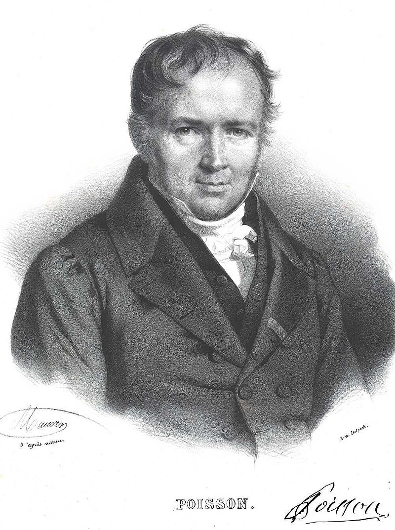
Figure 1: “Les Poissons”
Siméon Denis Poisson


Exercise 1 Define the Poisson distribution.


Solution 1.

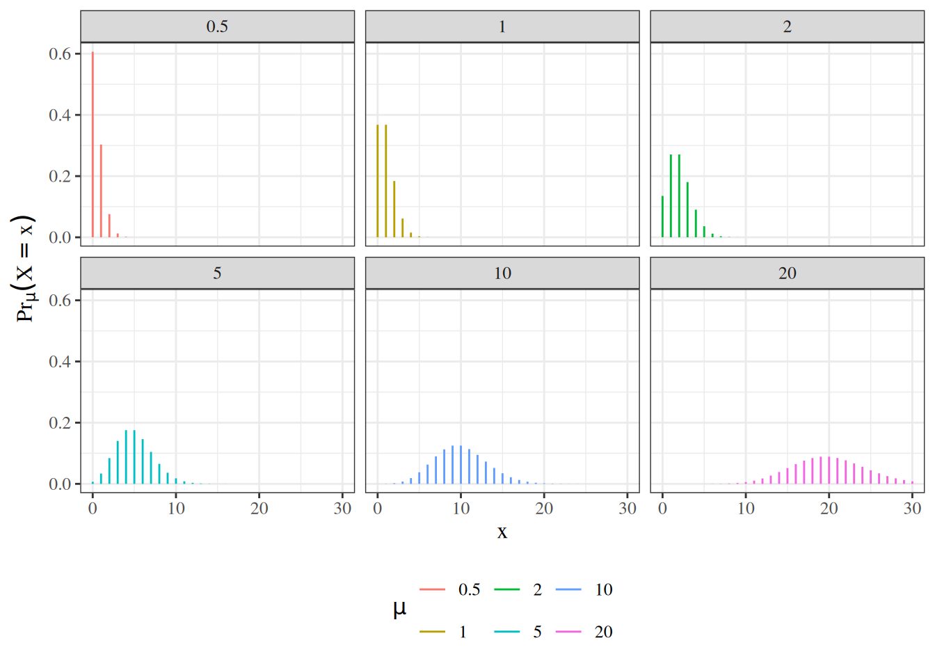
Definition 4 (Poisson distribution) \[\operatorname{P}(Y = y) = \frac{\mu^{y} e^{-\mu}}{y!}, y \in \mathbb{N} \tag{1}\]

(see Figure 2)


Exercise 2 What is the range of possible values for a Poisson distribution?


Solution 2. \[\mathcal{R}(Y) = \mathopen{}\left\{0, 1, 2, ...\right\}\mathclose{} = \mathbb{N}\]


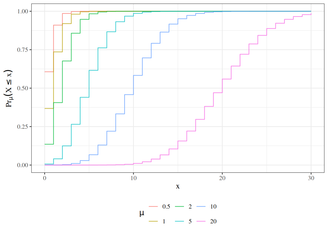
Theorem 6 (CDF of Poisson distribution) \[\operatorname{P}(Y \le y) = e^{-\mu} \sum_{j=0}^{\mathopen{}\left\lfloor y\right\rfloor\mathclose{}}\frac{\mu^j}{j!} \tag{2}\]

(see Figure 3)


Show R code
library(dplyr)
pois_dists <- tibble(
  mu = c(0.5, 1, 2, 5, 10, 20)
) |>
  reframe(
    .by = mu,
    x = 0:30
  ) |>
  mutate(
    `P(X = x)` = dpois(x, lambda = mu),
    `P(X <= x)` = ppois(x, lambda = mu),
    mu = factor(mu)
  )

library(ggplot2)
library(latex2exp)

plot0 <- pois_dists |>
  ggplot(
    aes(
      x = x,
      y = `P(X = x)`,
      fill = mu,
      col = mu
    )
  ) +
  theme(legend.position = "bottom") +
  labs(
    fill = latex2exp::TeX("$\\mu$"),
    col = latex2exp::TeX("$\\mu$"),
    y = latex2exp::TeX("$\\Pr_{\\mu}(X = x)$")
  )

plot1 <- plot0 +
  geom_segment(yend = 0) +
  facet_wrap(~mu)

print(plot1)
Figure 2: Poisson PMFs, by mean parameter \(\mu\)

Show R code
library(ggplot2)

plot2 <-
  plot0 +
  geom_step(alpha = 0.75) +
  aes(y = `P(X <= x)`) +
  labs(y = latex2exp::TeX("$\\Pr_{\\mu}(X \\leq x)$"))

print(plot2)
Figure 3: Poisson CDFs

Exercise 3 (Poisson distribution functions) Let \(X \sim \operatorname{Pois}(\mu = 3.75)\).

Compute:

  • \(\operatorname{P}(X = 4 | \mu = 3.75)\)
  • \(\operatorname{P}(X \le 7 | \mu = 3.75)\)
  • \(\operatorname{P}(X > 5 | \mu = 3.75)\)

Solution.

  • \(\operatorname{P}(X=4) = 0.19378\)
  • \(\operatorname{P}(X\le 7) = 0.962379\)
  • \(\operatorname{P}(X > 5) = 0.177117\)

Theorem 7 (Properties of the Poisson distribution) If \(X \sim \operatorname{Pois}(\mu)\), then:

  • \(\operatorname{E}[X] = \mu\)
  • \(\operatorname{Var}(X) = \mu\)
  • \(\operatorname{P}(X=x) = \frac{\mu}{x} \operatorname{P}(X = x-1)\)
  • For \(x < \mu\), \(\operatorname{P}(X=x) > \operatorname{P}(X = x-1)\)
  • For \(x = \mu\), \(\operatorname{P}(X=x) = \operatorname{P}(X = x-1)\)
  • For \(x > \mu\), \(\operatorname{P}(X=x) < \operatorname{P}(X = x-1)\)
  • \(\arg \max_{x} \operatorname{P}(X=x) = \mathopen{}\left\lfloor\mu\right\rfloor\mathclose{}\)

Exercise 4 Prove Theorem 7.


Solution. \[ \begin{aligned} \text{E}[X] &= \sum_{x=0}^\infty x \cdot P(X=x)\\ &= 0 \cdot P(X=0) + \sum_{x=1}^\infty x \cdot P(X=x)\\ &= 0 + \sum_{x=1}^\infty x \cdot P(X=x)\\ &= \sum_{x=1}^\infty x \cdot P(X=x)\\ &= \sum_{x=1}^\infty x \cdot \frac{\lambda^x e^{-\lambda}}{x!}\\ &= \sum_{x=1}^\infty x \cdot \frac{\lambda^x e^{-\lambda}}{x \cdot (x-1)!} & [\text{definition of factorial ("!") function}]\\ &= \sum_{x=1}^\infty \frac{\lambda^x e^{-\lambda}}{ (x-1)!}\\ &= \sum_{x=1}^\infty \frac{(\lambda \cdot \lambda^{x-1}) e^{-\lambda}}{ (x-1)!}\\ &= \lambda \cdot \sum_{x=1}^\infty \frac{( \lambda^{x-1}) e^{-\lambda}}{ (x-1)!}\\ &= \lambda \cdot \sum_{y=0}^\infty \frac{( \lambda^{y}) e^{-\lambda}}{ (y)!} &[\text{substituting } y \stackrel{\text{def}}{=}x-1]\\ &= \lambda \cdot 1 &[\text{because PDFs sum to 1}]\\ &= \lambda\\ \end{aligned} \]

See also https://statproofbook.github.io/P/poiss-mean.

For the variance, see https://statproofbook.github.io/P/poiss-var.


Accounting for exposure

Definition 5 (Exposure magnitude) For many count outcomes, there is some sense of an exposure magnitude, such as population size, or duration of observation, which multiplicatively rescales the expected (mean) count.


Exercise 5 What are some examples of exposure magnitudes?


Solution.

Table 3: Examples of exposure units
outcome exposure units
disease incidence number of individuals exposed; time at risk
car accidents miles driven
worksite accidents person-hours worked
population size size of habitat

Exposure units are similar to the number of trials in a binomial distribution, but in non-binomial count outcomes, there can be more than one event per unit of exposure.

We can use \(t\) to represent continuous-valued exposures/observation durations, and \(n\) to represent discrete-valued exposures.


Definition 6 (Event rate)  

For a count outcome \(Y\) with exposure magnitude \(t\), the event rate (denoted \(\lambda\)) is defined as the mean of \(Y\) divided by the exposure magnitude. That is:

\[\mu \stackrel{\text{def}}{=}\operatorname{E}[Y|T=t]\]

\[\lambda \stackrel{\text{def}}{=}\frac{\mu}{t} \tag{3}\]

Event rate is somewhat analogous to odds in binary outcome models; it typically serves as an intermediate transformation between the mean of the outcome and the linear component of the model. However, in contrast with the odds function, the transformation \(\lambda = \mu/t\) is not considered part of the Poisson model’s link function, and it treats the exposure magnitude covariate differently from the other covariates.


Theorem 8 (Transformation function from event rate to mean) For a count variable with mean \(\mu\), event rate \(\lambda\), and exposure magnitude \(t\):

\[\mu = \lambda \cdot t \tag{4}\]


Solution. Start from definition of event rate and use algebra to solve for \(\mu\).


Equation 4 is analogous to the inverse-odds function for binary variables.


Theorem 9 (No exposure means no expected events) When the exposure magnitude is 0, there is no opportunity for events to occur:

\[\operatorname{E}[Y|T=0] = 0\]


Proof. \[\operatorname{E}[Y|T=0] = \lambda \cdot 0 = 0\]


Important

The exposure magnitude, \(T\), is similar to a covariate in linear or logistic regression. However, there is an important difference: in count regression, there is no intercept corresponding to \(\operatorname{E}[Y|T=0]\). In other words, this model assumes that if there is no exposure, there can’t be any events.

Theorem 10 (Exposure is additive on the log scale) If \(\mu = \lambda\cdot t\), then:

\[\log{\mu} = \log{\lambda} + \log{t}\]

Definition 7 (Offset) When the linear component of a model involves a term without an unknown coefficient, that term is called an offset.


Theorem 11 (Sum of independent Poisson random variables) If \(X\) and \(Y\) are independent Poisson random variables with means \(\mu_X\) and \(\mu_Y\), their sum, \(Z=X+Y\), is also a Poisson random variable, with mean \(\mu_Z = \mu_X + \mu_Y\).


2.3 The Negative-Binomial distribution

Definition 8 (Negative binomial distribution) \[ \operatorname{P}(Y=y) = \frac{\mu^y}{y!} \cdot \frac{\Gamma(\rho + y)}{\Gamma(\rho) \cdot (\rho + \mu)^y} \cdot \left(1+\frac{\mu}{\rho}\right)^{-\rho} \]

where \(\rho\) is an overdispersion parameter and \(\Gamma(x) = (x-1)!\) for integers \(x\).

You don’t need to memorize or understand this expression.

As \(\rho \rightarrow \infty\), the second term converges to 1 and the third term converges to \(\operatorname{exp}\mathopen{}\left\{-\mu\right\}\mathclose{}\), which brings us back to the Poisson distribution.


Theorem 12 (Mean and variance of the negative binomial distribution) If \(Y \sim \operatorname{NegBin}(\mu, \rho)\), then:

  • \(\operatorname{E}[Y] = \mu\)
  • \(\operatorname{Var}\mathopen{}\left(Y\right)\mathclose{} = \mu + \frac{\mu^2}{\rho} > \mu\)

2.4 Weibull Distribution

\[ \begin{aligned} p(t)&= \alpha\lambda x^{\alpha-1}\text{e}^{-\lambda x^\alpha}\\ {\lambda}(t)&=\alpha\lambda x^{\alpha-1}\\ \operatorname{S}(t)&=\text{e}^{-\lambda x^\alpha}\\ E(T)&= \Gamma(1+1/\alpha)\cdot \lambda^{-1/\alpha} \end{aligned} \]

When \(\alpha=1\) this is the exponential. When \(\alpha>1\) the hazard is increasing and when \(\alpha < 1\) the hazard is decreasing. This provides more flexibility than the exponential.

We will see more of this distribution later.

3 Characteristics of probability distributions

3.1 Probability density function

Definition 9 (probability density) If \(X\) is a continuous random variable, then the probability density of \(X\) at value \(x\), denoted \(f(x)\), \(f_X(x)\), \(\operatorname{p}(x)\), \(\operatorname{p}_X(x)\), or \(\operatorname{p}(X=x)\), is defined as the limit of the probability (mass) that \(X\) is in an interval around \(x\), divided by the width of that interval, as that width reduces to 0.

\[ \begin{aligned} f(x) &\stackrel{\text{def}}{=}\lim_{\Delta \rightarrow 0} \frac{\operatorname{P}(X \in [x, x + \Delta])}{\Delta} \end{aligned} \]

See also Rothman et al. (2021) (Chapter 22, p. 535) and https://en.wikipedia.org/wiki/Probability_density_function#Formal_definition


Definition 10 (Cumulative distribution function (CDF)) For a random variable \(X\), its population CDF is \[F(t)=\Pr(X\le t), \quad t\in\mathbb{R}.\]

Definition 11 (Quantile function (population inverse CDF)) For a random variable \(X\) with cumulative distribution function (CDF) \(F\), its population quantile function (generalized inverse of \(F\)) is \[Q(p)=\inf\{t:F(t)\ge p\}, \quad 0<p\le 1.\]


Theorem 13 (Density function is derivative of CDF) The density function \(f(t)\) or \(\operatorname{p}(T=t)\) for a random variable \(T\) at value \(t\) is equal to the derivative of the cumulative probability function \(F(t) \stackrel{\text{def}}{=}P(T\le t)\); that is:

\[f(t) \stackrel{\text{def}}{=}\frac{\partial}{\partial t} F(t)\]


Theorem 14 (Density functions integrate to 1) For any density function \(f(x)\),

\[\int_{x \in \mathcal{R}(X)} f(x) dx = 1\]


3.2 Hazard function

Definition 12 (Hazard function, hazard rate, hazard rate function)  

The hazard function, hazard rate, hazard rate function, for a random variable \(T\) at value \(t\), typically denoted as \(\text{h}(t)\) 1 or \(\lambda(t)\), 2 is the conditional density of \(T\) at \(t\), given \(T \ge t\). That is:

\[{\lambda}(t) \stackrel{\text{def}}{=}\operatorname{p}(T=t|T\ge t)\]

If \(T\) represents the time at which an event occurs, then \({\lambda}(t)\) is the probability that the event occurs at time \(t\), given that it has not occurred prior to time \(t\).

The name “hazard” carries a connotation that the event is undesirable — death, relapse, equipment failure, etc. When the event in question is neutral or desirable (recovery, conception, graduation, response to treatment), the same quantity \({\lambda}(t)\) is often called the event incidence rate instead. This is parallel to the convention that conditional probabilities of undesirable events are called risks, while the same conditional probabilities for neutral/desirable events are simply called probabilities. The math is identical; only the name changes with the valence of the event.


Table 4: Probability distribution functions
Name Symbols Definition
Probability density function (PDF) \(\operatorname{f}(t), \operatorname{p}(t)\) \(\operatorname{p}(T=t)\)
Cumulative distribution function (CDF) \(\operatorname{F}(t), \operatorname{P}(t)\) \(\operatorname{P}(T\leq t)\)
Survival function \(\operatorname{S}(t), \bar{\operatorname{F}}(t)\) \(\operatorname{P}(T > t)\)
Hazard function \(\lambda(t), \operatorname{h}(t)\) \(\operatorname{p}(T=t|T\ge t)\)
Cumulative hazard function \(\Lambda(t), \operatorname{H}(t)\) \(\int_{u=-\infty}^t {\lambda}(u)du\)
Log-hazard function \(\eta(t)\) \(\operatorname{log}\mathopen{}\left\{{\lambda}(t)\right\}\mathclose{}\)

\[ \operatorname{f}(t) \xleftarrow[\operatorname{S}(t){\lambda}(t)]{-S'(t)} \operatorname{S}(t) \xleftarrow[]{\operatorname{exp}\mathopen{}\left\{-{\Lambda}(t)\right\}\mathclose{}} {\Lambda}(t) \xleftarrow[]{\int_{u=0}^t {\lambda}(u)du} {\lambda}(t) \xleftarrow[]{\operatorname{exp}\mathopen{}\left\{\eta(t)\right\}\mathclose{}} \eta(t) \]

\[ \operatorname{f}(t) \xrightarrow[\int_{u=t}^\infty \operatorname{f}(u)du]{\operatorname{f}(t)/{\lambda}(t)} \operatorname{S}(t) \xrightarrow[-\log{\operatorname{S}(t)}]{} {\Lambda}(t) \xrightarrow[{\Lambda}'(t)]{} {\lambda}(t) \xrightarrow[\operatorname{log}\mathopen{}\left\{{\lambda}(t)\right\}\mathclose{}]{} \eta(t) \]


3.3 Expectation

Definition 13 (Expectation, expected value, population mean ) The expectation, expected value, or population mean of a continuous random variable \(X\), denoted \(\operatorname{E}\mathopen{}\left[X\right]\mathclose{}\), \(\mu(X)\), or \(\mu_X\), is the weighted mean of \(X\)’s possible values, weighted by the probability density function of those values:

\[\operatorname{E}\mathopen{}\left[X\right]\mathclose{} = \int_{x\in \mathcal{R}(X)} x \cdot \operatorname{p}(X=x)dx\]

The expectation, expected value, or population mean of a discrete random variable \(X\), denoted \(\operatorname{E}\mathopen{}\left[X\right]\mathclose{}\), \(\mu(X)\), or \(\mu_X\), is the mean of \(X\)’s possible values, weighted by the probability mass function of those values:

\[\operatorname{E}\mathopen{}\left[X\right]\mathclose{} = \sum_{x \in \mathcal{R}(X)} x \cdot \operatorname{P}(X=x)\]

(c.f. https://en.wikipedia.org/wiki/Expected_value)


Theorem 15 (Expectation of the Bernoulli distribution) The expectation of a Bernoulli random variable with parameter \(\pi\) is:

\[\operatorname{E}\mathopen{}\left[X\right]\mathclose{} = \pi\]


Proof. \[ \begin{aligned} \operatorname{E}\mathopen{}\left[X\right]\mathclose{} &= \sum_{x\in \mathcal{R}(X)} x \cdot\operatorname{P}(X=x) \\&= \sum_{x\in \mathopen{}\left\{0,1\right\}\mathclose{}} x \cdot\operatorname{P}(X=x) \\&= \mathopen{}\left(0 \cdot\operatorname{P}(X=0)\right)\mathclose{} + \mathopen{}\left(1 \cdot\operatorname{P}(X=1)\right)\mathclose{} \\&= \mathopen{}\left(0 \cdot(1-\pi)\right)\mathclose{} + \mathopen{}\left(1 \cdot\pi\right)\mathclose{} \\&= 0 + \pi \\&= \pi \end{aligned} \]


Theorem 16 (Expectation of time-to-event variables) If \(T\) is a non-negative random variable, then:

\[\mu(T|\tilde{X}= \tilde{x}) = \int_{t=0}^{\infty}\operatorname{S}(t)dt\]

Proof. We prove the continuous case, in which \(T\) has a density \(\operatorname{f}\). The result follows from applying Tonelli’s theorem (hypothesis (a) of Fubini–Tonelli) to the function \(g(t, u) = \operatorname{f}(u) \cdot \mathbb{1}\mathopen{}\left(0 \le t \le u\right)\mathclose{}\) on the product space \([0, \infty) \times [0, \infty)\): \(g\) is nonnegative everywhere and vanishes outside the (unbounded) triangular region \(D = \{(t, u) : 0 \le t \le u < \infty\}\), so the iterated integrals over \(D\) are exchangeable.

Since \(\operatorname{f}(u) \ge 0\), hypothesis (a) of Fubini–Tonelli (the nonnegative case, Tonelli’s theorem) applies, and we may exchange the order of integration over \(D\):

\[ \begin{aligned} \operatorname{E}\mathopen{}\left[T\right]\mathclose{} &= \int_{u=0}^{\infty} u\,\operatorname{f}(u)\,du\\ &= \int_{u=0}^{\infty}\mathopen{}\left(\int_{t=0}^{u} 1\,dt\right)\mathclose{}\operatorname{f}(u)\,du\\ &= \int_{u=0}^{\infty}\int_{t=0}^{u} \operatorname{f}(u)\,dt\,du\\ &= \int_{t=0}^{\infty}\int_{u=t}^{\infty} \operatorname{f}(u)\,du\,dt\\ &= \int_{t=0}^{\infty}\operatorname{P}(T>t)\,dt\\ &= \int_{t=0}^{\infty}\operatorname{S}(t)\,dt. \end{aligned} \]

Exm

Example 3 (Mean of an exponential random variable via survival function) Let \(T \sim \mathrm{Exponential}(\lambda)\), so \(\operatorname{S}(t) = \text{e}^{-\lambda t}\) for \(t \ge 0\). By Theorem 16:

\[ \begin{aligned} \operatorname{E}\mathopen{}\left[T\right]\mathclose{} &= \int_0^\infty \operatorname{S}(t)\,dt\\ &= \int_0^\infty \text{e}^{-\lambda t}\,dt\\ &= \mathopen{}\left[-\frac{1}{\lambda}\text{e}^{-\lambda t}\right]\mathclose{}_0^\infty\\ &= \frac{1}{\lambda}, \end{aligned} \]

confirming the standard result \(\operatorname{E}\mathopen{}\left[T\right]\mathclose{} = 1/\lambda\).


Theorem 17 (Law of the Unconscious Statistician (LOTUS)) Discrete case. For any function \(g\) of a discrete random variable \(X\):

\[\operatorname{E}\mathopen{}\left[g(X)\right]\mathclose{} = \sum_{x \in \mathcal{R}(X)} g(x) \cdot\operatorname{P}(X=x)\]

Continuous case. For any function \(g\) of a continuous random variable \(X\) with density \(\operatorname{p}(X=x)\):

\[\operatorname{E}\mathopen{}\left[g(X)\right]\mathclose{} = \int_{x \in \mathcal{R}(X)} g(x) \cdot\operatorname{p}(X=x)\, dx\]


Proof. We prove the discrete case.

Let \(Y = g(X)\). By Definition 13 applied to \(Y\):

\[ \begin{aligned} \operatorname{E}\mathopen{}\left[g(X)\right]\mathclose{} &= \operatorname{E}\mathopen{}\left[Y\right]\mathclose{} \\&= \sum_{y \in \mathcal{R}(Y)} y \cdot\operatorname{P}(Y=y) \\&= \sum_{y \in \mathcal{R}(Y)} y \cdot\operatorname{P}(g(X)=y) \\&= \sum_{y \in \mathcal{R}(Y)} y \cdot\sum_{\substack{x \in \mathcal{R}(X) \\ g(x) = y}} \operatorname{P}(X=x) \\&= \sum_{x \in \mathcal{R}(X)} g(x) \cdot\operatorname{P}(X=x) \end{aligned} \]

where the last equality follows by rearranging the double sum, grouping each term \(x\) by its image \(y = g(x)\).

The continuous case is the density-weighted analogue of this argument, but a fully rigorous proof needs the general change-of-variables theorem for integrals against a pushforward measure — approximating \(g\) by simple functions and passing to the limit — which is beyond Epi 204’s scope (Billingsley 1995; Gut 2013; Casella and Berger 2002; Wikipedia contributors 2026).


LOTUS says that to compute \(\operatorname{E}\mathopen{}\left[g(X)\right]\mathclose{}\), we do not need to first find the distribution of \(g(X)\); we can compute the expectation directly using the distribution of \(X\).


Exm

Example 4 (Expected value of \(X^2\) for a Bernoulli variable) Let \(X \sim \operatorname{Ber}(\pi)\). By LOTUS (Theorem 17, discrete case):

\[ \begin{aligned} \operatorname{E}\mathopen{}\left[X^2\right]\mathclose{} &= \sum_{x \in \mathopen{}\left\{0,1\right\}\mathclose{}} x^2 \cdot\operatorname{P}(X=x) \\&= 0^2 \cdot\operatorname{P}(X=0) + 1^2 \cdot\operatorname{P}(X=1) \\&= 0^2 \cdot(1-\pi) + 1^2 \cdot\pi \\&= 0 + \pi \\&= \pi \end{aligned} \]


Exm

Example 5 (Expected value of \(X^2\) for a Uniform(0,1) variable) Let \(X \sim \text{Uniform}(0,1)\), so \(\operatorname{p}(X=x) = 1\) for \(x \in [0,1]\). By LOTUS (Theorem 17, continuous case):

\[ \begin{aligned} \operatorname{E}\mathopen{}\left[X^2\right]\mathclose{} &= \int_0^1 x^2 \cdot\operatorname{p}(X=x)\,dx && \text{(LOTUS, continuous case)} \\&= \int_0^1 x^2 \cdot 1\,dx && \text{(}\operatorname{p}(X=x) = 1\text{ on } [0,1]\text{)} \\&= \mathopen{}\left[\frac{x^3}{3}\right]\mathclose{}_0^1 && \text{(antiderivative of } x^2\text{)} \\&= \frac{1}{3}. && \text{(evaluate at the bounds)} \end{aligned} \]


3.3.1 Conditional distributions and expectations

Definition 14 (Conditional probability mass function) Let \(X\) and \(Y\) be jointly distributed discrete random variables. The conditional probability mass function of \(Y\) given \(X = x\) (for values of \(x\) with \(\operatorname{P}(X = x) > 0\)) is:

\[\operatorname{P}(Y = y \mid X = x) \stackrel{\text{def}}{=}\frac{\operatorname{P}(X = x,\, Y = y)}{\operatorname{P}(X = x)}\]


Exm

Example 6 (Conditional PMF from a vaccine trial) The vaccine dataset in the dobson package (Dobson and Barnett (2018), Table 9.6) records the response to treatment in a vaccine trial: \(X\) is treatment group (placebo or vaccine) and \(Y\) is response severity (small, moderate, or large).

Show R code
library(dobson)
library(dplyr)
data(vaccine)
response_levels <- c("small", "moderate", "large")
vaccine_tab <- vaccine |>
  mutate(response = factor(response, levels = response_levels)) |>
  xtabs(frequency ~ treatment + response, data = _)
pander::pander(as.data.frame.matrix(vaccine_tab))
  small moderate large
placebo 25 8 5
vaccine 6 18 11

The joint PMF of \((X, Y)\) is the table of frequencies divided by the total \(n = 73\) trial participants. The marginal probability \(\operatorname{P}(X = \text{placebo})\) is:

\[ \begin{aligned} \operatorname{P}(X = \text{placebo}) &= \operatorname{P}(X = \text{placebo},\, Y = \text{small}) + \operatorname{P}(X = \text{placebo},\, Y = \text{moderate}) + \operatorname{P}(X = \text{placebo},\, Y = \text{large}) \\&= \tfrac{25}{73} + \tfrac{8}{73} + \tfrac{5}{73} \\&= \tfrac{38}{73} \end{aligned} \]

By Definition 14, the conditional PMF of \(Y\) given \(X = \text{placebo}\) is:

\[ \begin{aligned} \operatorname{P}(Y = \text{small} \mid X = \text{placebo}) &= \frac{\operatorname{P}(X = \text{placebo},\, Y = \text{small})}{\operatorname{P}(X = \text{placebo})} \\&= \frac{25/73}{38/73} \\&= \frac{25}{38} \end{aligned} \]


Definition 15 (Conditional probability density function) Let \(X\) and \(Y\) be jointly distributed continuous random variables with joint density \(\operatorname{p}(X = x,\, Y = y)\) and marginal density \(\operatorname{p}(X = x)\). The conditional probability density function of \(Y\) given \(X = x\) (for values of \(x\) with \(\operatorname{p}(X = x) > 0\)) is:

\[\operatorname{p}(Y = y \mid X = x) \stackrel{\text{def}}{=}\frac{\operatorname{p}(X = x,\, Y = y)}{\operatorname{p}(X = x)}\]


Exm

Example 7 (Conditional PDF from a bivariate normal model of birthweight data) The birthweight dataset in the dobson package (Dobson and Barnett (2018), Table 2.3) records gestational age (weeks) and birthweight (grams) for 12 boys and 12 girls. Let \(X\) be gestational age and \(Y\) be birthweight, pooling both sexes into \(n = 24\) observations.

Show R code
library(dobson)
data(birthweight)
ga <- c(birthweight[["boys gestational age"]],
        birthweight[["girls gestational age"]])
wt <- c(birthweight[["boys weight"]], birthweight[["girls weight"]])
mu_x <- mean(ga)
sigma_x <- sd(ga)
mu_y <- mean(wt)
sigma_y <- sd(wt)
rho <- cor(ga, wt)
beta <- cov(ga, wt) / var(ga)
intercept <- mu_y - beta * mu_x
x0 <- 40
marg_dens_x0 <- dnorm(x0, mean = mu_x, sd = sigma_x)
cond_mean <- intercept + beta * x0
cond_sd <- sigma_y * sqrt(1 - rho^2)
pander::pander(data.frame(
  parameter = c("mu_x", "sigma_x", "mu_y", "sigma_y", "rho"),
  estimate = round(c(mu_x, sigma_x, mu_y, sigma_y, rho), 4)
))
parameter estimate
mu_x 38.54
sigma_x 1.817
mu_y 2,968
sigma_y 282.1
rho 0.7443

Modeling \((X, Y)\) as bivariate normal with parameters set equal to these sample moments, the joint density is (a standard result; e.g. Casella and Berger (2002)):

\[ \operatorname{p}(X=x,\,Y=y) = \frac{1}{2\pi\sigma_X\sigma_Y\sqrt{1-\rho^2}} \text{e}^{-\frac{1}{2(1-\rho^2)} \mathopen{}\left[\frac{(x-\mu_X)^2}{\sigma_X^2} - \frac{2\rho(x-\mu_X)(y-\mu_Y)}{\sigma_X\sigma_Y} + \frac{(y-\mu_Y)^2}{\sigma_Y^2}\right]\mathclose{}} \]

A further standard fact about the bivariate normal (Casella and Berger (2002)) is that the marginal distribution of \(X\) is \(X \sim \operatorname{N}\mathopen{}\left(\mu_X, \sigma_X^2\right)\mathclose{}\). At \(x = 40\) weeks (a full-term pregnancy), \(\mu_X = 38.5417\) and \(\sigma_X = 1.8173\), so:

\[ \begin{aligned} \operatorname{p}(X=40) &= \frac{1}{\sigma_X\sqrt{2\pi}} \text{e}^{-\frac{(40-\mu_X)^2}{2\sigma_X^2}} \\&= \frac{1}{1.8173\sqrt{2\pi}} \text{e}^{-\frac{(40-38.5417)^2}{2(1.8173)^2}} \\&\approx 0.1591 \end{aligned} \]

By Definition 15, dividing the joint density by this marginal density and simplifying the exponent (completing the square in \(y\); Casella and Berger (2002)) gives the conditional PDF of \(Y\) given \(X = 40\), which is itself normal with mean shifted along the regression line and variance reduced by a factor of \(1-\rho^2\):

\[ \begin{aligned} \operatorname{p}(Y=y \mid X=40) &= \frac{\operatorname{p}(X=40,\,Y=y)}{\operatorname{p}(X=40)} \\&= \frac{1}{\sigma_Y\sqrt{2\pi(1-\rho^2)}} \text{e}^{-\frac{1}{2(1-\rho^2)}\mathopen{}\left[\frac{(40-\mu_X)^2}{\sigma_X^2} - \frac{2\rho(40-\mu_X)(y-\mu_Y)}{\sigma_X\sigma_Y} + \frac{(y-\mu_Y)^2}{\sigma_Y^2}\right]\mathclose{} + \frac{(40-\mu_X)^2}{2\sigma_X^2}} \\&= \frac{1}{\sigma_Y\sqrt{2\pi(1-\rho^2)}} \text{e}^{-\frac{\rho^2(40-\mu_X)^2}{2\sigma_X^2(1-\rho^2)} + \frac{\rho(40-\mu_X)(y-\mu_Y)}{\sigma_X\sigma_Y(1-\rho^2)} - \frac{(y-\mu_Y)^2}{2\sigma_Y^2(1-\rho^2)}} \\&= \frac{1}{\sigma_Y\sqrt{2\pi(1-\rho^2)}} \text{e}^{-\frac{1}{2\sigma_Y^2(1-\rho^2)} \mathopen{}\left[\rho^2\frac{\sigma_Y^2}{\sigma_X^2}(40-\mu_X)^2 - 2\rho\frac{\sigma_Y}{\sigma_X}(40-\mu_X)(y-\mu_Y) + (y-\mu_Y)^2\right]\mathclose{}} \\&= \frac{1}{\sigma_Y\sqrt{2\pi(1-\rho^2)}} \text{e}^{-\frac{\mathopen{}\left(y - \mathopen{}\left[\mu_Y + \rho\frac{\sigma_Y}{\sigma_X}(40-\mu_X)\right]\mathclose{}\right)\mathclose{}^2}{2\sigma_Y^2(1-\rho^2)}} \end{aligned} \]

The first equality substitutes the joint and marginal densities and combines their prefactors and exponents; the second equality combines the two \((40-\mu_X)^2\) terms using \(1 - \tfrac{1}{1-\rho^2} = \tfrac{-\rho^2}{1-\rho^2}\); the third equality factors \(-\tfrac{1}{2\sigma_Y^2(1-\rho^2)}\) out of the bracket (multiplying through confirms it reproduces the previous line); and the fourth equality completes the square in \(y\), since expanding \(\mathopen{}\left(y - \mathopen{}\left[\mu_Y + \rho\frac{\sigma_Y}{\sigma_X}(40-\mu_X)\right]\mathclose{}\right)\mathclose{}^2\) reproduces exactly the bracketed quadratic in the third equality.

So \(Y \mid X = 40 \sim \operatorname{N}\mathopen{}\left(3136.15,\, 188.37^2\right)\mathclose{}\): the conditional mean, 3136.15 g, is exactly the fitted regression line’s prediction at \(x=40\) (\(-1484.9846 + 115.5283 \times 40 = 3136.15\)), matching R’s lm(wt ~ ga) fit directly:

Show R code
pander::pander(coef(lm(wt ~ ga)))
(Intercept) ga
-1,485 115.5

Definition 16 (Conditional expectation) Discrete case. Let \(X\) and \(Y\) be jointly distributed discrete random variables. The conditional expectation of \(Y\) given \(X = x\), using Definition 14, is:

\[\operatorname{E}\mathopen{}\left[Y \mid X = x\right]\mathclose{} \stackrel{\text{def}}{=}\sum_{y \in \mathcal{R}(Y)} y \cdot\operatorname{P}(Y = y \mid X = x)\]

Continuous case. Let \(X\) and \(Y\) be jointly distributed continuous random variables. The conditional expectation of \(Y\) given \(X = x\), using Definition 15, is:

\[\operatorname{E}\mathopen{}\left[Y \mid X = x\right]\mathclose{} \stackrel{\text{def}}{=}\int_{y \in \mathcal{R}(Y)} y \cdot\operatorname{p}(Y = y \mid X = x)\, dy\]


Exm

Example 8 (Conditional expectation from real trial and birthweight data) Discrete case. Continuing Example 6, score the vaccine trial’s response levels \(\text{small} = 1\), \(\text{moderate} = 2\), \(\text{large} = 3\). The conditional PMF of \(Y\) given \(X = \text{placebo}\) (from Example 6) is:

\[ \begin{aligned} \operatorname{P}(Y = \text{small} \mid X = \text{placebo}) &= \tfrac{25}{38} \\ \operatorname{P}(Y = \text{moderate} \mid X = \text{placebo}) &= \tfrac{8}{38} \\ \operatorname{P}(Y = \text{large} \mid X = \text{placebo}) &= \tfrac{5}{38} \end{aligned} \]

so:

\[ \begin{aligned} \operatorname{E}\mathopen{}\left[Y \mid X = \text{placebo}\right]\mathclose{} &= 1 \cdot\tfrac{25}{38} + 2 \cdot\tfrac{8}{38} + 3 \cdot\tfrac{5}{38} \\&= \frac{25 + 16 + 15}{38} \\&= \frac{56}{38} \\&= \frac{28}{19} \\&\approx 1.47 \end{aligned} \]

Continuous case. Continuing Example 7, \(Y \mid X = 40 \sim \operatorname{N}\mathopen{}\left(3136.15,\, 188.37^2\right)\mathclose{}\). Since the mean of a normal random variable is its own location parameter, integrating \(y\) against this conditional density directly gives:

\[ \begin{aligned} \operatorname{E}\mathopen{}\left[Y \mid X = 40\right]\mathclose{} &= \int_{-\infty}^{\infty} y \cdot\operatorname{p}(Y=y \mid X=40)\,dy \\&= 3136.15 \text{ g} \end{aligned} \]

matching the fitted regression line’s prediction at \(x=40\) weeks exactly, as expected since the conditional mean of a bivariate normal is the linear regression of \(Y\) on \(X\).


Definition 17 (Conditional expectation: mixed case) Suppose exactly one of \(X, Y\) is discrete and the other is continuous. Write \(\operatorname{p}(X = x,\, Y = y)\) for their joint density-mass function: a probability density in the continuous variable and a probability mass in the discrete variable.

\(X\) discrete, \(Y\) continuous. Here \(\operatorname{p}(X=x,\,Y=y)\) is, for each fixed \(x\), a probability density in \(y\), scaled so that \(\int_{y} \operatorname{p}(X=x,\,Y=y)\,dy = \operatorname{P}(X=x)\). The conditional PDF of \(Y\) given \(X = x\) (for values of \(x\) with \(\operatorname{P}(X = x) > 0\)) is:

\[\operatorname{p}(Y = y \mid X = x) \stackrel{\text{def}}{=}\frac{\operatorname{p}(X = x,\, Y = y)}{\operatorname{P}(X = x)}\]

and the conditional expectation of \(Y\) given \(X = x\) is:

\[\operatorname{E}\mathopen{}\left[Y \mid X = x\right]\mathclose{} \stackrel{\text{def}}{=}\int_{y \in \mathcal{R}(Y)} y \cdot\operatorname{p}(Y = y \mid X = x)\, dy\]

\(X\) continuous, \(Y\) discrete. Here \(\operatorname{p}(X=x,\,Y=y)\) is, for each fixed \(y\), a probability density in \(x\), scaled so that \(\sum_{y} \operatorname{p}(X=x,\,Y=y) = \operatorname{p}(X=x)\). The conditional PMF of \(Y\) given \(X = x\) (for values of \(x\) with \(\operatorname{p}(X = x) > 0\)) is:

\[\operatorname{P}(Y = y \mid X = x) \stackrel{\text{def}}{=}\frac{\operatorname{p}(X = x,\, Y = y)}{\operatorname{p}(X = x)}\]

and the conditional expectation of \(Y\) given \(X = x\) is:

\[\operatorname{E}\mathopen{}\left[Y \mid X = x\right]\mathclose{} \stackrel{\text{def}}{=}\sum_{y \in \mathcal{R}(Y)} y \cdot\operatorname{P}(Y = y \mid X = x)\]


Exm

Example 9 (Conditional expectation, one discrete variable and one continuous variable) \(X\) discrete, \(Y\) continuous. The plasma dataset in the dobson package (Dobson and Barnett (2018), Table 6.25) records plasma inorganic phosphate levels (mg/dL) one hour after a glucose tolerance test, for hyperinsulinemic obese (H-O) and control (C) participants. Let \(X\) be group and \(Y\) be phosphate level.

Show R code
library(dobson)
library(dplyr)
data(plasma)
plasma_subset <- plasma |> filter(Group %in% c("H-O", "C"))
plasma_summary <- plasma_subset |>
  summarise(n = n(), mean = mean(phosphate), sd = sd(phosphate), .by = Group)
n_ho <- plasma_summary$n[plasma_summary$Group == "H-O"]
n_c <- plasma_summary$n[plasma_summary$Group == "C"]
mean_ho <- plasma_summary$mean[plasma_summary$Group == "H-O"]
sd_ho <- plasma_summary$sd[plasma_summary$Group == "H-O"]
mean_c <- plasma_summary$mean[plasma_summary$Group == "C"]
sd_c <- plasma_summary$sd[plasma_summary$Group == "C"]
pander::pander(plasma_summary)
Group n mean sd
H-O 11 3.945 0.7776
C 12 2.783 0.4086

Modeling phosphate as approximately normal within each group, with parameters set equal to each group’s sample mean and SD, and \(\operatorname{P}(X = \text{H-O}) = 11/23\):

\[\operatorname{p}(Y = y \mid X = \text{H-O}) \approx \operatorname{N}\mathopen{}\left(3.95,\, 0.78^2\right)\mathclose{}\] \[\operatorname{p}(Y = y \mid X = \text{C}) \approx \operatorname{N}\mathopen{}\left(2.78,\, 0.41^2\right)\mathclose{}\]

By Definition 17, since the mean of a normal random variable is its own location parameter:

\[\operatorname{E}\mathopen{}\left[Y \mid X = \text{H-O}\right]\mathclose{} = 3.95 \text{ mg/dL}, \qquad \operatorname{E}\mathopen{}\left[Y \mid X = \text{C}\right]\mathclose{} = 2.78 \text{ mg/dL}\]

\(X\) continuous, \(Y\) discrete. The senility dataset in the dobson package (Dobson and Barnett (2018), Table 7.8) records, for 54 elderly people, a WAIS (Wechsler Adult Intelligence Scale) score and whether symptoms of senility were present. Let \(X\) be WAIS score and \(Y\) indicate senility symptoms.

Show R code
data(senility)
senility_fit <- glm(s ~ x, data = senility, family = binomial)
b0 <- coef(senility_fit)[["(Intercept)"]]
b1 <- coef(senility_fit)[["x"]]
pander::pander(coef(senility_fit))
(Intercept) x
2.404 -0.3235

Modeling \(\operatorname{P}(Y = 1 \mid X = x)\) with the fitted logistic regression:

\[\operatorname{logit}\operatorname{P}(Y = 1 \mid X = x) = 2.4040 - 0.3235\, x\]

By Definition 17, since \(Y \mid X=x\) is Bernoulli:

\[ \begin{aligned} \operatorname{E}\mathopen{}\left[Y \mid X = x\right]\mathclose{} &= 0 \cdot\operatorname{P}(Y=0 \mid X=x) + 1 \cdot\operatorname{P}(Y=1 \mid X=x) \\&= \operatorname{P}(Y=1 \mid X=x) \\&= \frac{1}{1 + \text{e}^{-(2.4040 - 0.3235\, x)}} \end{aligned} \]

Show R code
senility_p10 <- predict(senility_fit,
                        newdata = data.frame(x = 10), type = "response")
senility_p15 <- predict(senility_fit,
                        newdata = data.frame(x = 15), type = "response")

At \(x = 10\): \(\operatorname{E}\mathopen{}\left[Y \mid X=10\right]\mathclose{} = 0.3\). At \(x = 15\): \(\operatorname{E}\mathopen{}\left[Y \mid X=15\right]\mathclose{} = 0.08\) — a lower WAIS score is associated with higher predicted probability of senility symptoms.


Definition 18 (Conditional expectation function) The conditional expectation function \(\operatorname{E}\mathopen{}\left[Y \mid X\right]\mathclose{}\) is the function (and hence random variable) of \(X\) obtained by evaluating \(\operatorname{E}\mathopen{}\left[Y \mid X = x\right]\mathclose{}\) at \(X\); that is, \(\operatorname{E}\mathopen{}\left[Y \mid X\right]\mathclose{} = g(X)\) where \(g(x) \stackrel{\text{def}}{=}\operatorname{E}\mathopen{}\left[Y \mid X = x\right]\mathclose{}\).


Exm

Example 10 (The conditional expectation function of the birthweight model) Continuing Example 7 and Example 8, \((X, Y)\) (gestational age, birthweight) is modeled as bivariate normal. The general form of the conditional mean derived in Example 7, evaluated at an arbitrary \(x\) instead of just \(x=40\), gives the conditional expectation function directly:

\[ \begin{aligned} g(x) &= \mu_Y + \rho\frac{\sigma_Y}{\sigma_X}(x-\mu_X) \\&= -1484.9846 + 115.5283\, x \end{aligned} \]

which is exactly the fitted regression line (the general algebraic identity \(\mu_Y + \rho\frac{\sigma_Y}{\sigma_X}(x-\mu_X) = \mathopen{}\left(\mu_Y - \rho\frac{\sigma_Y}{\sigma_X}\mu_X\right)\mathclose{} + \rho\frac{\sigma_Y}{\sigma_X}x\) is what makes the bivariate-normal conditional mean linear in \(x\)).

As a check, evaluating at \(x = 40\) recovers Example 8’s result:

\[g(40) = -1484.9846 + 115.5283 \times 40 = 3136.15 \text{ g}\]

Exercise 6 (Expectation of a sum, given a joint PMF) Let \((X, Y)\) be discrete with joint probability mass function:

\(Y = 0\) \(Y = 1\)
\(X = 0\) \(0.2\) \(0.3\)
\(X = 1\) \(0.1\) \(0.4\)

Compute \(\operatorname{E}\mathopen{}\left[X + Y\right]\mathclose{}\).

Solution. Treating \((X, Y)\) as a single discrete random object taking one of the four values \((0,0)\), \((0,1)\), \((1,0)\), \((1,1)\), LOTUS (Theorem 17) applied to \(g(x, y) = x + y\) gives directly:

\[ \begin{aligned} \operatorname{E}\mathopen{}\left[X + Y\right]\mathclose{} &= \sum_{x \in \{0,1\}} \sum_{y \in \{0,1\}} (x + y)\,\operatorname{P}(X = x,\, Y = y) \\ &= (0{+}0)(0.2) + (0{+}1)(0.3) + (1{+}0)(0.1) + (1{+}1)(0.4) \\ &= 0 + 0.3 + 0.1 + 0.8 \\ &= 1.2 \end{aligned} \]

As a check: \(\operatorname{E}\mathopen{}\left[X\right]\mathclose{} = 0(0.5) + 1(0.5) = 0.5\) and \(\operatorname{E}\mathopen{}\left[Y\right]\mathclose{} = 0(0.3) + 1(0.7) = 0.7\), so \(\operatorname{E}\mathopen{}\left[X + Y\right]\mathclose{} = \operatorname{E}\mathopen{}\left[X\right]\mathclose{} + \operatorname{E}\mathopen{}\left[Y\right]\mathclose{} = 1.2\).

Show R code
x_labs <- c("X=0", "X=0", "X=1", "X=1")
y_labs <- c("Y=0", "Y=1", "Y=0", "Y=1")
probs <- c(0.2, 0.3, 0.1, 0.4)

plotly::plot_ly(
  x = ~y_labs, y = ~probs, color = ~x_labs,
  colors = c("steelblue", "tomato"),
  type = "bar"
) |>
  plotly::layout(
    barmode = "group",
    xaxis = list(title = "Y"),
    yaxis = list(title = "P(X = x, Y = y)", range = c(0, 0.5)),
    legend = list(title = list(text = "X value"))
  )
Figure 4: Joint probability mass function \(\operatorname{P}(X = x, Y = y)\). Marginal totals: \(\operatorname{P}(X = 0) = 0.5\), \(\operatorname{P}(X = 1) = 0.5\), \(\operatorname{P}(Y = 0) = 0.3\), \(\operatorname{P}(Y = 1) = 0.7\).

Note that \(X\) and \(Y\) are not independent here: \(\operatorname{P}(X = 0, Y = 0) = 0.2 \neq 0.15 = \operatorname{P}(X = 0)\,\operatorname{P}(Y = 0)\). LOTUS applies regardless, since it requires only the actual joint mass function, not independence.

There are only four \((x,y)\) pairs here, so summing them in any order — row by row, column by column, or any other listing — gives the same total by ordinary commutativity and associativity of addition; no result about interchanging summation order is needed. Fubini–Tonelli, covered next, is what’s needed once the support is countably infinite instead — see Exercise 7.

3.4 Fubini–Tonelli for expectations

The Riemann version of Fubini’s theorem, stated in the math-prereqs chapter, lets us switch the order of integration for continuous integrands on simple regions. For expectations against probability measures we use its measure-theoretic form, which holds on any σ-finite measure space. The σ-finiteness hypothesis is automatic for probability measures (every probability measure is finite, hence σ-finite), so Fubini–Tonelli yields the corollary below directly.

Corollary 3 (Joint-distribution form (without independence; corollary of Fubini–Tonelli)) Let \((X, Y)\) be jointly distributed random variables whose joint distribution has a density \(f_{X,Y}\) with respect to a product of σ-finite reference measures \(\mu_X \otimes \mu_Y\) on \(\mathcal{R}(X) \times \mathcal{R}(Y)\), and let \(h : \mathcal{R}(X) \times \mathcal{R}(Y) \to \mathbb{R}\) be measurable. If either

  1. \(h(X, Y) \ge 0\) almost surely, or

  2. \(\operatorname{E}\mathopen{}\left[\mathopen{}\left|h(X, Y)\right|\mathclose{}\right]\mathclose{} < \infty\),

then the expectation of \(h(X, Y)\) can be written as an iterated integral against \(f_{X,Y}\), with the order of integration exchangeable:

\[ \begin{aligned} \operatorname{E}\mathopen{}\left[h(X, Y)\right]\mathclose{} &= \int_{\mathcal{R}(X)}\mathopen{}\left(\int_{\mathcal{R}(Y)} h(x, y)\,f_{X,Y}(x, y)\,d\mu_Y(y)\right)\mathclose{}\,d\mu_X(x) \\&= \int_{\mathcal{R}(Y)}\mathopen{}\left(\int_{\mathcal{R}(X)} h(x, y)\,f_{X,Y}(x, y)\,d\mu_X(x)\right)\mathclose{}\,d\mu_Y(y). \end{aligned} \]

The choice of reference measures covers three cases:

  • Both continuous: \(\mu_X = \mu_Y = \text{Lebesgue measure}\); \(f_{X,Y}\) is the joint probability density function (PDF), and \(\int g(x)\,d\mu_X(x) = \int g(x)\,dx\).
  • Both discrete: \(\mu_X = \mu_Y = \text{counting measure}\); \(f_{X,Y}(x,y) = \operatorname{P}(X = x,\, Y = y)\) is the joint probability mass function (PMF), and \(\int g(x)\,d\mu_X(x) = \sum_{x \in \mathcal{R}(X)} g(x)\).
  • Mixed (one continuous, one discrete): one reference measure is Lebesgue and the other is counting; \(f_{X,Y}(x,y) = f_{X \mid Y}(x \mid y)\,\operatorname{P}(Y = y)\) (or \(\operatorname{P}(X = x \mid Y = y)\,f_Y(y)\) if \(X\) is discrete and \(Y\) continuous), and the iterated integrals combine an ordinary integral with a sum. The conditional densities/PMFs here are defined the same way as in Definition 17, just conditioning on \(Y\) instead of \(X\).

Proof. Apply Fubini–Tonelli with \(\mu_1 = \mu_X\) and \(\mu_2 = \mu_Y\) to the integrand \(h(x,y)\,f_{X,Y}(x,y)\) on \(\mathcal{R}(X) \times \mathcal{R}(Y)\). Lebesgue measure and counting measure on a countable set are each σ-finite, so \(\mu_X \otimes \mu_Y\) is σ-finite in all three cases. The relevant hypothesis is (a) when \(h \ge 0\) and (b) when \(\operatorname{E}\mathopen{}\left[\mathopen{}\left|h(X, Y)\right|\mathclose{}\right]\mathclose{} < \infty\). Independence is not required. When \(X\) and \(Y\) are independent, \(f_{X,Y}(x,y) = f_X(x)\,f_Y(y)\) (or \(\operatorname{P}(X=x,Y=y) = \operatorname{P}(X=x)\,\operatorname{P}(Y=y)\) in the discrete case), and the iterated integrals factor into separate integrals over the marginals.

Exm

Example 11 (Expectation of a product of independent variables) Let \(X \sim \mathrm{Uniform}(0, 1)\) and \(Y \sim \mathrm{Uniform}(0, 2)\), independently distributed. Compute \(\operatorname{E}\mathopen{}\left[XY\right]\mathclose{}\).

We apply Corollary 3 (both-continuous case) with \(h(x, y) = xy\). Since \(X\) and \(Y\) are independent with densities \(f_X(x) = 1\) on \([0,1]\) and \(f_Y(y) = \tfrac{1}{2}\) on \([0,2]\), the joint density factors as \(f_{X,Y}(x,y) = f_X(x)\,f_Y(y) = \tfrac{1}{2}\), and \(\mu_X = \mu_Y = \text{Lebesgue measure}\):

\[ \begin{aligned} \operatorname{E}\mathopen{}\left[XY\right]\mathclose{} &= \int_0^1 \mathopen{}\left(\int_0^2 xy \cdot\tfrac{1}{2}\,dy\right)\mathclose{}\,dx \\&= \int_0^1 x\mathopen{}\left(\frac{1}{2}\int_0^2 y\,dy\right)\mathclose{}\,dx \\&= \int_0^1 x \cdot\frac{1}{2} \cdot\mathopen{}\left[\frac{y^2}{2}\right]\mathclose{}_0^2\,dx \\&= \int_0^1 x \cdot\frac{1}{2} \cdot 2\,dx \\&= \int_0^1 x\,dx \\&= \frac{1}{2} \end{aligned} \]

As a check: \(\operatorname{E}\mathopen{}\left[X\right]\mathclose{} = \tfrac{1}{2}\), \(\operatorname{E}\mathopen{}\left[Y\right]\mathclose{} = 1\), and \(\operatorname{E}\mathopen{}\left[X\right]\mathclose{}\operatorname{E}\mathopen{}\left[Y\right]\mathclose{} = \tfrac{1}{2}\).

Exm

Example 12 (When independence fails: a counterexample) Correctly applying Corollary 3 requires the actual joint density \(f_{X,Y}\) — not the product of marginals \(f_X(x)\,f_Y(y)\), which is valid only when \(X\) and \(Y\) are independent. Using the wrong joint density gives the wrong answer.

Let \(X \sim \mathrm{Uniform}(0, 1)\) and set \(Y = X\) (so \(X\) and \(Y\) are perfectly correlated and not independent).

True expectation:

\[ \operatorname{E}\mathopen{}\left[XY\right]\mathclose{} = \operatorname{E}\mathopen{}\left[X \cdot X\right]\mathclose{} = \operatorname{E}\mathopen{}\left[X^2\right]\mathclose{} = \int_0^1 x^2\,dx = \frac{1}{3} \]

Erroneously applying the product-measure formula:

Note that Fubini–Tonelli’s own conditions still hold here (\(h(x,y) = xy\) is nonnegative and integrable), so the error is not a failure of Fubini–Tonelli. Rather, the error is using the wrong measure: the joint distribution of \((X, X)\) is concentrated on the diagonal \(\{(x, x) : x \in [0, 1]\} \subset [0, 1]^2\), which has Lebesgue measure zero in \(\mathbb{R}^2\). The joint distribution is therefore not absolutely continuous with respect to two-dimensional Lebesgue measure, so no joint density \(f_{X,Y}\) on \([0, 1]^2\) exists, which is the reference density Corollary 3 requires.

The calculation below is what someone would erroneously write if they assumed independence and used \(f_X(x)\,f_Y(y)\) as a “joint density” — a function that does not in fact correspond to the joint distribution of \((X, X)\). The marginals \(X \sim \mathrm{Uniform}(0,1)\) and \(Y \sim \mathrm{Uniform}(0,1)\) do have densities \(f_X = f_Y = 1\), but the product \(f_X(x)\,f_Y(y) = 1\) on \([0, 1]^2\) is the density of an independent pair, not of \((X, X)\):

\[ \begin{aligned} \int_0^1\!\int_0^1 xy \cdot f_X(x) \cdot f_Y(y)\,dy\,dx &= \int_0^1\!\int_0^1 xy\,dy\,dx \\&= \int_0^1 x\mathopen{}\left(\int_0^1 y\,dy\right)\mathclose{}\,dx \\&= \int_0^1 x \cdot\frac{1}{2}\,dx \\&= \frac{1}{4} \end{aligned} \]

This recovers \(\operatorname{E}\mathopen{}\left[XY\right]\mathclose{}\) for independent uniforms (\(\tfrac{1}{4}\)), not \(\operatorname{E}\mathopen{}\left[XX\right]\mathclose{}\) for the perfectly correlated pair (\(\tfrac{1}{3}\)). The lesson is that Corollary 3 requires the actual joint density \(f_{X,Y}\). For independent \((X, Y)\), this factors as \(f_X(x)\,f_Y(y)\); for dependent \((X, Y)\), \(f_{X,Y}\) need not factor — and for \((X, X)\), no joint density on \(\mathbb{R}^2\) exists at all, so Corollary 3 simply does not apply.

Show R code
set.seed(204)
n <- 400
x_dep <- runif(n)
y_dep <- x_dep
x_ind <- runif(n)
y_ind <- runif(n)

plotly::plot_ly() |>
  plotly::add_trace(
    type = "scatter", mode = "markers",
    x = x_ind, y = y_ind,
    name = "Assumed independent (X<sub>1</sub>, X<sub>2</sub>)",
    marker = list(size = 5, color = "#999999", opacity = 0.5)
  ) |>
  plotly::add_trace(
    type = "scatter", mode = "markers",
    x = x_dep, y = y_dep,
    name = "Actual (X, X) on diagonal",
    marker = list(size = 6, color = "#b40426")
  ) |>
  plotly::layout(
    xaxis = list(title = "x", range = c(0, 1), scaleanchor = "y"),
    yaxis = list(title = "y", range = c(0, 1)),
    legend = list(orientation = "h", y = -0.2)
  )
Figure 5: Samples from the joint distribution of \((X, X)\) (red, on the diagonal) versus an independent pair \((X_1, X_2)\) with the same marginals (grey, scattered over \([0, 1]^2\)). The actual joint mass for \((X, X)\) is concentrated on a 1-dimensional diagonal — a set of Lebesgue measure zero in \(\mathbb{R}^2\) — so no joint density on \([0, 1]^2\) exists, and the “\(f_X(x)\,f_Y(y) = 1\)” calculation integrates against the wrong measure (the grey distribution).
Exm

Example 13 (Both-continuous case: joint PDF on a non-rectangular support) Let \((X, Y)\) have joint density \(f_{X,Y}(x, y) = 2\) for \(0 \le x \le y \le 1\) (and \(0\) otherwise). Compute \(\operatorname{E}\mathopen{}\left[X + Y\right]\mathclose{}\).

By Corollary 3:

\[ \begin{aligned} \operatorname{E}\mathopen{}\left[X + Y\right]\mathclose{} &= \int_0^1\!\int_0^y (x + y) \cdot 2\,dx\,dy \\&= 2\int_0^1 \mathopen{}\left[\frac{x^2}{2} + xy\right]\mathclose{}_{x=0}^{x=y}\,dy \\&= 2\int_0^1 \mathopen{}\left(\frac{y^2}{2} + y^2\right)\mathclose{}\,dy \\&= 2\int_0^1 \frac{3y^2}{2}\,dy \\&= 3\int_0^1 y^2\,dy \\&= 3 \cdot\frac{1}{3} \\&= 1 \end{aligned} \]

Show R code
n_grid <- 51
x_seq <- seq(0, 1, length.out = n_grid)
y_seq <- seq(0, 1, length.out = n_grid)

z_mat <- outer(x_seq, y_seq, function(x, y) {
  z <- rep(2, length(x))
  z[x > y] <- NA
  z
})

plotly::plot_ly(x = ~x_seq, y = ~y_seq, z = ~t(z_mat)) |>
  plotly::add_surface(showscale = FALSE) |>
  plotly::layout(scene = list(
    xaxis = list(title = "x"),
    yaxis = list(title = "y"),
    zaxis = list(title = "f(x, y)", range = c(0, 2.5)),
    camera = list(eye = list(x = 1.6, y = -1.6, z = 0.8))
  ))
Figure 6: Joint density \(f_{X,Y}(x, y) = 2\) on the triangular support \(\{(x, y) : 0 \le x \le y \le 1\}\), and zero elsewhere. The total “volume” under the density is \(2 \cdot \tfrac{1}{2} = 1\), as required.

Exercise 7 (Both-discrete case, infinite support: joint PMF) Let \(X\) and \(Y\) be independent, each Geometric on \(\mathcal{R}(X) = \mathcal{R}(Y) = \{0, 1, 2, \dots\}\) with \(\operatorname{P}(X = x) = (1-p)\,p^x\) for a fixed \(p \in (0, 1)\) (\(X\) counts the number of failures before the first success in a sequence of independent trials with success probability \(1-p\); likewise for \(Y\)). Unlike Exercise 6, the support here is countably infinite. The joint PMF is \(\operatorname{P}(X = x,\, Y = y) = (1-p)^2\,p^{x+y}\).

Compute \(\operatorname{E}\mathopen{}\left[X + Y\right]\mathclose{}\).

Solution. Compute \(\operatorname{E}\mathopen{}\left[X + Y\right]\mathclose{}\) using Corollary 3 with \(\mu_X = \mu_Y = \text{counting measure}\) and \(h(x, y) = x + y\). Since \(h(x,y) = x + y \ge 0\) for every \((x,y)\) in this support, hypothesis (a) holds, so Corollary 3 (via Tonelli’s theorem) guarantees the order of this now-infinite double sum is exchangeable — unlike the finite case, elementary algebra alone could not establish this.

By Corollary 3 (both-discrete case), summing over \(y\) first for each fixed \(x\):

\[ \begin{aligned} \operatorname{E}\mathopen{}\left[X + Y\right]\mathclose{} &= \sum_{x=0}^{\infty} \sum_{y=0}^{\infty} (x + y)\,\operatorname{P}(X = x,\, Y = y) \\&= \sum_{x=0}^{\infty} \sum_{y=0}^{\infty} (x + y)(1-p)^2 p^{x+y} \\&= \sum_{x=0}^{\infty} (1-p)^2 p^x \sum_{y=0}^{\infty} (x + y)\,p^y \\&= \sum_{x=0}^{\infty} (1-p)^2 p^x \mathopen{}\left(x \sum_{y=0}^{\infty} p^y + \sum_{y=0}^{\infty} y\,p^y\right)\mathclose{} \\&= \sum_{x=0}^{\infty} (1-p)^2 p^x \mathopen{}\left(\frac{x}{1-p} + \frac{p}{(1-p)^2}\right)\mathclose{} \\&= \sum_{x=0}^{\infty} p^x \mathopen{}\left[x(1-p) + p\right]\mathclose{} \\&= (1-p) \sum_{x=0}^{\infty} x\,p^x + p \sum_{x=0}^{\infty} p^x \\&= (1-p) \cdot\frac{p}{(1-p)^2} + p \cdot\frac{1}{1-p} \\&= \frac{p}{1-p} + \frac{p}{1-p} \\&= \frac{2p}{1-p} \end{aligned} \]

using the standard geometric-series facts \(\sum_{y=0}^{\infty} p^y = \frac{1}{1-p}\) and \(\sum_{y=0}^{\infty} y\,p^y = \frac{p}{(1-p)^2}\) (e.g. Casella and Berger (2002)).

As a check, \(\operatorname{E}\mathopen{}\left[X\right]\mathclose{} = \operatorname{E}\mathopen{}\left[Y\right]\mathclose{} = \frac{p}{1-p}\) (the mean of this Geometric distribution; Casella and Berger (2002)), so \(\operatorname{E}\mathopen{}\left[X + Y\right]\mathclose{} = \operatorname{E}\mathopen{}\left[X\right]\mathclose{} + \operatorname{E}\mathopen{}\left[Y\right]\mathclose{} = \frac{2p}{1-p}\) by linearity, matching.

Show R code
p <- 0.4
exact_sum <- 2 * p / (1 - p)

n_trunc <- 500
support <- 0:n_trunc
joint_pmf_fn <- function(x, y) (1 - p)^2 * p^(x + y)
joint_probs <- outer(support, support, joint_pmf_fn)
h_vals <- outer(support, support, function(x, y) x + y)

sum_y_first <- sum(rowSums(h_vals * joint_probs))
sum_x_first <- sum(colSums(h_vals * joint_probs))

pander::pander(data.frame(
  quantity = c("exact (closed form)", "sum over y first, then x",
               "sum over x first, then y"),
  value = round(c(exact_sum, sum_y_first, sum_x_first), 6)
))
quantity value
exact (closed form) 1.333
sum over y first, then x 1.333
sum over x first, then y 1.333

With \(p = 0.4\), summing \(y\) first then \(x\), and summing \(x\) first then \(y\), agree with each other and with the closed form \(\frac{2p}{1-p} = 1.3333\) up to truncation error — exactly Tonelli’s guarantee.

NoteTonelli’s nonnegativity condition, and what happens without it

The example above only needed hypothesis (a), \(h(X,Y) \ge 0\), because \(h(x,y) = x+y\) is nonnegative on this support. For a signed \(h\), interchanging an infinite double sum is not automatically valid — Corollary 3’s hypothesis (b), \(\operatorname{E}\mathopen{}\left[\mathopen{}\left|h(X,Y)\right|\mathclose{}\right]\mathclose{} < \infty\), is what licenses it in that case. Without either hypothesis, the two orders can genuinely disagree. A standard example (a signed array, not a probability distribution; see e.g. Rudin (1976) for the general theory of rearranging series): let \(a_{m,n} = 1\) if \(m = n\), \(a_{m,n} = -1\) if \(m = n+1\), and \(a_{m,n} = 0\) otherwise, for \(m, n = 0, 1, 2, \dots\). Summing each row \(m\) first: row \(0\) has only the term \(a_{0,0}=1\) (there is no valid \(n = -1\)), so its row sum is \(1\); every row \(m \ge 1\) has \(a_{m,m} = 1\) and \(a_{m,m-1} = -1\), so its row sum is \(0\). Summing the rows then gives \(1 + 0 + 0 + \cdots = 1\). Summing each column \(n\) first: every column \(n \ge 0\) has \(a_{n,n} = 1\) and \(a_{n+1,n} = -1\), so its column sum is always \(0\), and summing the columns then gives \(0 + 0 + \cdots = 0\). The two orders give \(1\) and \(0\): genuinely different answers, confirming that a condition like (a) or (b) really is needed once the terms are no longer all nonnegative.

Exercise 8 (Mixed case: one continuous variable, one discrete variable) Let \(Y \sim \mathrm{Bernoulli}(0.6)\) and, given \(Y = y\), let \(X \mid Y = y \sim \mathrm{Uniform}(0,\, y + 1)\).

Compute \(\operatorname{E}\mathopen{}\left[X\right]\mathclose{}\).

Solution. Compute \(\operatorname{E}\mathopen{}\left[X\right]\mathclose{}\) using Corollary 3 with \(\mu_X = \text{Lebesgue measure}\), \(\mu_Y = \text{counting measure}\), and \(h(x, y) = x\).

The joint density w.r.t. Lebesgue \(\times\) counting measure is \(f_{X,Y}(x, y) = f_{X \mid Y}(x \mid y)\,\operatorname{P}(Y = y)\):

\[ \begin{aligned} f_{X,Y}(x,\, 0) &= 1 \cdot 0.4 = 0.4 &&\text{ for } x \in [0,1];\\ f_{X,Y}(x,\, 1) &= \tfrac{1}{2} \cdot 0.6 = 0.3 &&\text{ for } x \in [0,2]. \end{aligned} \]

By Corollary 3 (mixed case):

\[ \begin{aligned} \operatorname{E}\mathopen{}\left[X\right]\mathclose{} &= \sum_{y \in \{0,1\}} \int_0^{y+1} x\,f_{X,Y}(x,\, y)\,dx \\ &= \int_0^1 x \cdot 0.4\,dx + \int_0^2 x \cdot 0.3\,dx \\ &= 0.4 \cdot \frac{1}{2} + 0.3 \cdot 2 \\ &= 0.2 + 0.6 = 0.8 \end{aligned} \]

As a check using the law of total expectation: \(\operatorname{E}\mathopen{}\left[X \mid Y = 0\right]\mathclose{} = \tfrac{1}{2}\) and \(\operatorname{E}\mathopen{}\left[X \mid Y = 1\right]\mathclose{} = 1\), so \(\operatorname{E}\mathopen{}\left[X\right]\mathclose{} = \tfrac{1}{2}(0.4) + 1(0.6) = 0.2 + 0.6 = 0.8\).

Show R code
x_fine <- seq(0, 2, by = 0.005)
df <- data.frame(
  x = c(x_fine[x_fine <= 1], x_fine),
  density = c(rep(0.4, sum(x_fine <= 1)), rep(0.3, length(x_fine))),
  label = c(
    rep("Y = 0  (P = 0.4)", sum(x_fine <= 1)),
    rep("Y = 1  (P = 0.6)", length(x_fine))
  )
)

plotly::plot_ly(
  df, x = ~x, y = ~density, color = ~label,
  colors = c("steelblue", "tomato")
) |>
  plotly::add_lines() |>
  plotly::layout(
    xaxis = list(title = "x"),
    yaxis = list(title = "f<sub>X,Y</sub>(x, y)", range = c(0, 0.55)),
    legend = list(title = list(text = "Y value"))
  )
Figure 7: Joint density \(f_{X,Y}(x, y) = f_{X \mid Y}(x \mid y)\,\operatorname{P}(Y = y)\) for each value of the discrete variable \(Y\). The area under each component integrates to \(\operatorname{P}(Y = y)\): \(0.4 \cdot 1 = 0.4\) (blue) and \(0.3 \cdot 2 = 0.6\) (red), summing to 1.

\(Y\) takes only finitely many values here (two), so \(\sum_{y \in \{0,1\}} \int_0^{y+1} x\,f_{X,Y}(x,\,y)\,dx\) is just linearity of the integral applied to a two-term sum — \(\int g + \int k = \int (g + k)\) — not a genuine interchange of summation and integration order. Exercise 9 below gives \(Y\) a countably infinite range instead, so the sum-of-integrals is genuinely infinite and Corollary 3’s guarantee is load-bearing.

Exercise 9 (Mixed case, infinite discrete support) Let \(Y\) be Geometric on \(\{0, 1, 2, \dots\}\) with \(\operatorname{P}(Y = y) = (1-q)\,q^y\) for a fixed \(q \in (0, 1)\) and, given \(Y = y\), let \(X \mid Y = y \sim \mathrm{Uniform}(0,\, y+1)\). Unlike Exercise 8, \(Y\)’s range here is countably infinite.

Compute \(\operatorname{E}\mathopen{}\left[X\right]\mathclose{}\).

Solution. Compute \(\operatorname{E}\mathopen{}\left[X\right]\mathclose{}\) using Corollary 3 with \(\mu_X = \text{Lebesgue measure}\), \(\mu_Y = \text{counting measure}\), and \(h(x, y) = x\).

The joint density w.r.t. Lebesgue \(\times\) counting measure is \(f_{X,Y}(x, y) = f_{X \mid Y}(x \mid y)\,\operatorname{P}(Y = y) = \frac{(1-q)\,q^y}{y+1}\) for \(x \in [0, y+1]\).

Since \(h(x, y) = x \ge 0\) on this support, hypothesis (a) holds, so Corollary 3 (via Tonelli’s theorem) guarantees the now-infinite sum-of-integrals below is valid — unlike Exercise 8, this is not simply linearity applied to a finite sum.

By Corollary 3 (mixed case):

\[ \begin{aligned} \operatorname{E}\mathopen{}\left[X\right]\mathclose{} &= \sum_{y=0}^{\infty} \int_0^{y+1} x\,f_{X,Y}(x,\,y)\,dx \\&= \sum_{y=0}^{\infty} \frac{(1-q)\,q^y}{y+1} \int_0^{y+1} x\,dx \\&= \sum_{y=0}^{\infty} \frac{(1-q)\,q^y}{y+1} \cdot\frac{(y+1)^2}{2} \\&= \frac{1-q}{2} \sum_{y=0}^{\infty} (y+1)\,q^y \\&= \frac{1-q}{2} \mathopen{}\left(\sum_{y=0}^{\infty} y\,q^y + \sum_{y=0}^{\infty} q^y\right)\mathclose{} \\&= \frac{1-q}{2} \mathopen{}\left(\frac{q}{(1-q)^2} + \frac{1}{1-q}\right)\mathclose{} \\&= \frac{1-q}{2} \cdot\frac{q + (1-q)}{(1-q)^2} \\&= \frac{1-q}{2} \cdot\frac{1}{(1-q)^2} \\&= \frac{1}{2(1-q)} \end{aligned} \]

using the same geometric-series facts as Exercise 7 (e.g. Casella and Berger (2002)).

As a check using the law of total expectation: \(\operatorname{E}\mathopen{}\left[X \mid Y=y\right]\mathclose{} = \frac{y+1}{2}\) (the mean of \(\mathrm{Uniform}(0,y+1)\)) and \(\operatorname{E}\mathopen{}\left[Y\right]\mathclose{} = \frac{q}{1-q}\) (the mean of this Geometric distribution; Casella and Berger (2002)), so:

\[ \begin{aligned} \operatorname{E}\mathopen{}\left[X\right]\mathclose{} &= \operatorname{E}\mathopen{}\left[\operatorname{E}\mathopen{}\left[X \mid Y\right]\mathclose{}\right]\mathclose{} \\&= \operatorname{E}\mathopen{}\left[\frac{Y+1}{2}\right]\mathclose{} \\&= \frac{\operatorname{E}\mathopen{}\left[Y\right]\mathclose{} + 1}{2} \\&= \frac{1}{2}\mathopen{}\left(\frac{q}{1-q} + 1\right)\mathclose{} \\&= \frac{1}{2} \cdot\frac{q + (1-q)}{1-q} \\&= \frac{1}{2(1-q)} \end{aligned} \]

matching.

Show R code
q <- 0.5
exact_ex <- 1 / (2 * (1 - q))

n_trunc <- 2000
y_vals <- 0:n_trunc
py_vals <- (1 - q) * q^y_vals
cond_mean <- (y_vals + 1) / 2
trunc_ex <- sum(cond_mean * py_vals)

pander::pander(data.frame(
  quantity = c("exact (closed form)", "truncated sum-of-integrals"),
  value = round(c(exact_ex, trunc_ex), 6)
))
quantity value
exact (closed form) 1
truncated sum-of-integrals 1

With \(q = 0.5\), the truncated sum-of-integrals matches the closed form \(\frac{1}{2(1-q)} = 1\).


Theorem 18 (Law of iterated expectations) For any two random variables \(X\) and \(Y\):

\[\operatorname{E}\mathopen{}\left[Y\right]\mathclose{} = \operatorname{E}\mathopen{}\left[\operatorname{E}\mathopen{}\left[Y \mid X\right]\mathclose{}\right]\mathclose{}\]

Alternate names for this identity include: the tower rule, the tower property, the law of total expectation, and the smoothing theorem.


Proof. Discrete case. When \(X\) and \(Y\) are discrete, applying Definition 13 to \(\operatorname{E}\mathopen{}\left[\operatorname{E}\mathopen{}\left[Y \mid X\right]\mathclose{}\right]\mathclose{}\) and then the law of total probability (Theorem 4) applied to the countable partition \(\{X = x : x \in \mathcal{R}(X)\}\):

\[ \begin{aligned} \operatorname{E}\mathopen{}\left[\operatorname{E}\mathopen{}\left[Y \mid X\right]\mathclose{}\right]\mathclose{} &= \sum_{x \in \mathcal{R}(X)} \operatorname{E}\mathopen{}\left[Y \mid X=x\right]\mathclose{} \cdot\operatorname{P}(X=x) \\&= \sum_{x \in \mathcal{R}(X)} \mathopen{}\left(\sum_{y \in \mathcal{R}(Y)} y \cdot\operatorname{P}(Y=y \mid X=x)\right)\mathclose{} \cdot\operatorname{P}(X=x) \\&= \sum_{y \in \mathcal{R}(Y)} y \cdot\sum_{x \in \mathcal{R}(X)} \operatorname{P}(Y=y \mid X=x) \cdot\operatorname{P}(X=x) \\&= \sum_{y \in \mathcal{R}(Y)} y \cdot\operatorname{P}(Y=y) \\&= \operatorname{E}\mathopen{}\left[Y\right]\mathclose{} \end{aligned} \]

Continuous case. When \(X\) and \(Y\) are continuous, applying Definition 13 to \(\operatorname{E}\mathopen{}\left[\operatorname{E}\mathopen{}\left[Y \mid X\right]\mathclose{}\right]\mathclose{}\) and then using Definition 16 for \(\operatorname{E}\mathopen{}\left[Y \mid X=x\right]\mathclose{}\):

\[ \begin{aligned} \operatorname{E}\mathopen{}\left[\operatorname{E}\mathopen{}\left[Y \mid X\right]\mathclose{}\right]\mathclose{} &= \int_{x \in \mathcal{R}(X)} \operatorname{E}\mathopen{}\left[Y \mid X=x\right]\mathclose{} \cdot\operatorname{p}(X=x)\, dx \\&= \int_{x \in \mathcal{R}(X)} \mathopen{}\left(\int_{y \in \mathcal{R}(Y)} y \cdot\operatorname{p}(Y=y \mid X=x)\, dy\right)\mathclose{} \cdot\operatorname{p}(X=x)\, dx \\&= \int_{y \in \mathcal{R}(Y)} y \cdot\mathopen{}\left(\int_{x \in \mathcal{R}(X)} \operatorname{p}(Y=y \mid X=x) \cdot\operatorname{p}(X=x)\, dx\right)\mathclose{}\, dy \\&= \int_{y \in \mathcal{R}(Y)} y \cdot\operatorname{p}(Y=y)\, dy \\&= \operatorname{E}\mathopen{}\left[Y\right]\mathclose{} \end{aligned} \]

where the third equality exchanges the order of integration by hypothesis (b) of Fubini–Tonelli (the absolute-integrability case, Fubini’s theorem); this requires \(\operatorname{E}\mathopen{}\left[\mathopen{}\left|Y\right|\mathclose{}\right]\mathclose{} < \infty\), which is implicit in \(\operatorname{E}\mathopen{}\left[Y\right]\mathclose{}\) being defined, and the fourth equality uses \(\int_{x} \operatorname{p}(Y=y \mid X=x) \cdot\operatorname{p}(X=x)\, dx = \int_{x} \operatorname{p}(X=x, Y=y)\, dx = \operatorname{p}(Y=y)\) (marginalization of the joint density).


Theorem 19 (Conditional law of iterated expectations) For random variables \(X\), \(Y\), and \(Z\):

\[\operatorname{E}\mathopen{}\left[Y \mid Z\right]\mathclose{} = \operatorname{E}\mathopen{}\left[\operatorname{E}\mathopen{}\left[Y \mid X,Z\right]\mathclose{} \mid Z\right]\mathclose{}\]

This is the tower rule applied conditionally on \(Z\).


Proof. For each fixed value \(z\) with positive probability or density:

Discrete case. Conditioning on \(Z=z\), and applying the law of total probability to the partition \(\{X=x : x \in \mathcal{R}(X)\}\) under the conditional distribution given \(Z=z\):

\[ \begin{aligned} \operatorname{E}\mathopen{}\left[\operatorname{E}\mathopen{}\left[Y \mid X,Z\right]\mathclose{} \mid Z=z\right]\mathclose{} &= \sum_{x \in \mathcal{R}(X)} \operatorname{E}\mathopen{}\left[Y \mid X=x,Z=z\right]\mathclose{} \cdot\operatorname{P}(X=x \mid Z=z) \\&= \operatorname{E}\mathopen{}\left[Y \mid Z=z\right]\mathclose{} \end{aligned} \]

Continuous case. Conditioning on \(Z=z\), and integrating over \(X\) under the conditional density \(\operatorname{p}(X=x \mid Z=z)\):

\[ \begin{aligned} \operatorname{E}\mathopen{}\left[\operatorname{E}\mathopen{}\left[Y \mid X,Z\right]\mathclose{} \mid Z=z\right]\mathclose{} &= \int_{x \in \mathcal{R}(X)} \operatorname{E}\mathopen{}\left[Y \mid X=x,Z=z\right]\mathclose{} \cdot\operatorname{p}(X=x \mid Z=z)\, dx \\&= \operatorname{E}\mathopen{}\left[Y \mid Z=z\right]\mathclose{} \end{aligned} \]

Therefore, as random variables of \(Z\), \(\operatorname{E}\mathopen{}\left[Y \mid Z\right]\mathclose{} = \operatorname{E}\mathopen{}\left[\operatorname{E}\mathopen{}\left[Y \mid X,Z\right]\mathclose{} \mid Z\right]\mathclose{}\).


Exm

Example 14 (Marginal expectation from conditional expectations) Suppose \(X\) is a binary random variable indicating treatment assignment (\(X=1\) treated, \(X=0\) control), with \(\operatorname{P}(X=1) = 0.5\), and suppose the outcome \(Y\) has conditional expectations:

\[\operatorname{E}\mathopen{}\left[Y \mid X=1\right]\mathclose{} = 10, \quad \operatorname{E}\mathopen{}\left[Y \mid X=0\right]\mathclose{} = 6\]

By the law of iterated expectations (Theorem 18):

\[ \begin{aligned} \operatorname{E}\mathopen{}\left[Y\right]\mathclose{} &= \operatorname{E}\mathopen{}\left[\operatorname{E}\mathopen{}\left[Y \mid X\right]\mathclose{}\right]\mathclose{} \\&= \operatorname{E}\mathopen{}\left[Y \mid X=1\right]\mathclose{} \cdot\operatorname{P}(X=1) + \operatorname{E}\mathopen{}\left[Y \mid X=0\right]\mathclose{} \cdot\operatorname{P}(X=0) \\&= 10 \cdot 0.5 + 6 \cdot 0.5 \\&= 5 + 3 \\&= 8 \end{aligned} \]


Definition 19 (Expectation of a random matrix) For a random matrix \(\mathbf{A}\) of size \(m \times n\) with \((i,j)\)-th element \(A_{ij}\), the expectation \(\operatorname{E}\mathbf{A}\) is the \(m \times n\) matrix whose \((i,j)\)-th element is \(\operatorname{E}\mathopen{}\left[A_{ij}\right]\mathclose{}\):

\[ \operatorname{E}\mathbf{A} \stackrel{\text{def}}{=}\begin{pmatrix} \operatorname{E}\mathopen{}\left[A_{11}\right]\mathclose{} & \operatorname{E}\mathopen{}\left[A_{12}\right]\mathclose{} & \cdots & \operatorname{E}\mathopen{}\left[A_{1n}\right]\mathclose{} \\ \operatorname{E}\mathopen{}\left[A_{21}\right]\mathclose{} & \operatorname{E}\mathopen{}\left[A_{22}\right]\mathclose{} & \cdots & \operatorname{E}\mathopen{}\left[A_{2n}\right]\mathclose{} \\ \vdots & \vdots & \ddots & \vdots \\ \operatorname{E}\mathopen{}\left[A_{m1}\right]\mathclose{} & \operatorname{E}\mathopen{}\left[A_{m2}\right]\mathclose{} & \cdots & \operatorname{E}\mathopen{}\left[A_{mn}\right]\mathclose{} \end{pmatrix} \]

In other words, expectation is applied element-wise to a random matrix.


3.5 Deviation, error, and noise

Definition 20 (Deviation) A deviation is the difference between a value and a reference value. For any quantity \(z\) and reference value \(r\):

\[z - r\]

In probability and statistics, “deviation” often means deviation from a population mean. For a random variable \(Y\):

\[Y - \operatorname{E}\mathopen{}\left[Y\right]\mathclose{}\]

See: Wikipedia: Deviation (statistics)


Definition 21 (Deviation from a population or subpopulation mean) In probabilistic models, we call this quantity a deviation from a mean. It is often also called an error or noise term in other sources. For the random variable \(Y\), define the deviation from its mean as:

\[e(Y) \stackrel{\text{def}}{=}Y - \operatorname{E}\mathopen{}\left[Y\right]\mathclose{}\]

For a realized observation \(y\): \[e(y) \stackrel{\text{def}}{=}y - \operatorname{E}\mathopen{}\left[Y\right]\mathclose{}\]

In regression settings, the reference mean is often conditional on covariates: \(e(y_i) \stackrel{\text{def}}{=}y_i - \operatorname{E}\mathopen{}\left[Y_i \mid X_i\right]\mathclose{}\).

In this course, we prefer “deviation” for this mean-deviation quantity. The terms “error” and “noise” are common aliases. We use “residual” (defined in the Linear regression chapter) for deviations from fitted values. For notation in this course, we use \(e(\cdot)\) for these model/data deviations, and reserve \(\varepsilon\mathopen{}\left(\cdot\right)\mathclose{}\) for estimator-to-estimand deviations (see Estimation).

See:


3.7 The Central Limit Theorem

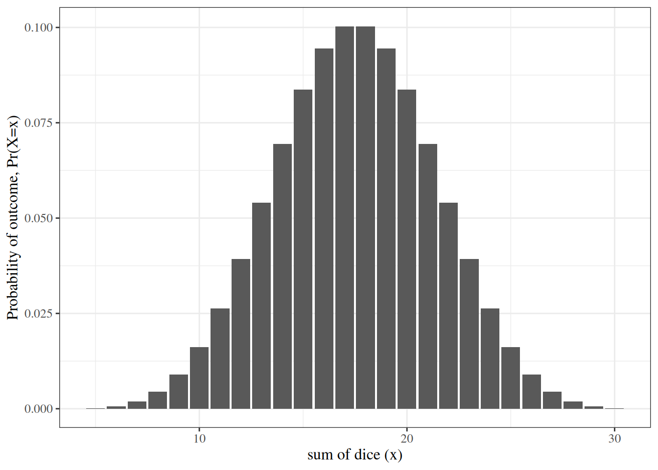
The sum of many independent or nearly-independent random variables with small variances (relative to the number of RVs being summed) produces bell-shaped distributions.

For example, consider the sum of five dice (Figure 8).

Show R code
library(dplyr)
dist = 
  expand.grid(1:6, 1:6, 1:6, 1:6, 1:6) |> 
  rowwise() |>
  mutate(total = sum(c_across(everything()))) |> 
  ungroup() |> 
  count(total) |> 
  mutate(`p(X=x)` = n/sum(n))

library(ggplot2)

dist |> 
  ggplot() +
  aes(x = total, y = `p(X=x)`) +
  geom_col() +
  xlab("sum of dice (x)") +
  ylab("Probability of outcome, Pr(X=x)") +
  expand_limits(y = 0)


Figure 8: Distribution of the sum of five dice

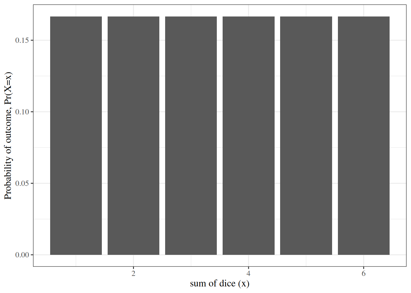
In comparison, the outcome of just one die is not bell-shaped (Figure 9).

Show R code
library(dplyr)
dist = 
  expand.grid(1:6) |> 
  rowwise() |>
  mutate(total = sum(c_across(everything()))) |> 
  ungroup() |> 
  count(total) |> 
  mutate(`p(X=x)` = n/sum(n))

library(ggplot2)

dist |> 
  ggplot() +
  aes(x = total, y = `p(X=x)`) +
  geom_col() +
  xlab("sum of dice (x)") +
  ylab("Probability of outcome, Pr(X=x)") +
  expand_limits(y = 0)


Figure 9: Distribution of the outcome of one die

What distribution does a single die have?

Answer: discrete uniform on 1:6.

4 Additional resources

References

Billingsley, Patrick. 1995. Probability and Measure. 3rd ed. Wiley Series in Probability and Mathematical Statistics. Wiley.
Casella, George, and Roger Berger. 2002. Statistical Inference. 2nd ed. Cengage Learning. https://www.cengage.com/c/statistical-inference-2e-casella-berger/9780534243128/.
Dobson, Annette J, and Adrian G Barnett. 2018. An Introduction to Generalized Linear Models. 4th ed. CRC press. https://doi.org/10.1201/9781315182780.
Gut, Allan. 2013. Probability: A Graduate Course. 2nd ed. Springer Texts in Statistics. Springer. https://doi.org/10.1007/978-1-4614-4708-5.
Kalbfleisch, John D, and Ross L Prentice. 2011. The Statistical Analysis of Failure Time Data. John Wiley & Sons.
Klein, John P, and Melvin L Moeschberger. 2003. Survival Analysis: Techniques for Censored and Truncated Data. Vol. 1230. Springer. https://link.springer.com/book/10.1007/b97377.
Kleinbaum, David G, and Mitchel Klein. 2012. Survival Analysis: A Self-Learning Text. 3rd ed. Springer. https://link.springer.com/book/10.1007/978-1-4419-6646-9.
Miller, Steven J. 2017. The Probability Lifesaver : All the Tools You Need to Understand Chance. A Princeton Lifesaver Study Guide. Princeton University Press. https://press.princeton.edu/books/hardcover/9780691149547/the-probability-lifesaver.
Rothman, Kenneth J., Timothy L. Lash, Tyler J. VanderWeele, and Sebastien Haneuse. 2021. Modern Epidemiology. Fourth edition. Wolters Kluwer.
Rudin, Walter. 1976. Principles of Mathematical Analysis. 3rd ed. International Series in Pure and Applied Mathematics. McGraw-Hill.
Vittinghoff, Eric, David V Glidden, Stephen C Shiboski, and Charles E McCulloch. 2012. Regression Methods in Biostatistics: Linear, Logistic, Survival, and Repeated Measures Models. 2nd ed. Springer. https://doi.org/10.1007/978-1-4614-1353-0.
Wikipedia contributors. 2026. Law of the Unconscious Statistician — Wikipedia, the Free Encyclopedia. https://en.wikipedia.org/wiki/Law_of_the_unconscious_statistician.
Back to top

Footnotes

  1. for example in Dobson and Barnett (2018), Vittinghoff et al. (2012), Klein and Moeschberger (2003), and Kleinbaum and Klein (2012)↩︎

  2. for example, in Rothman et al. (2021) and Kalbfleisch and Prentice (2011)↩︎