how-to-use-rwicc • rwicc

This vignette shows how to generate a simulated data set and analyze it using the model and estimation algorithm described in “Regression with Interval-Censored Covariates: Application to Cross-Sectional Incidence Estimation” by Morrison, Laeyendecker, and Brookmeyer (2021) in Biometrics: https://onlinelibrary.wiley.com/doi/10.1111/biom.13472.

First, we simulate some data:


set.seed(1)

library(rwicc)
library(dplyr)
#> 
#> Attaching package: 'dplyr'
#> The following objects are masked from 'package:stats':
#> 
#>     filter, lag
#> The following objects are masked from 'package:base':
#> 
#>     intersect, setdiff, setequal, union
library(ggplot2)
theta_true = c(0.986, -3.88)
hazard_alpha = 1
hazard_beta = 0.5
sim_data = simulate_interval_censoring(
  "theta" = theta_true,
  "study_cohort_size" = 4500,
  "preconversion_interval_length" = 365,
  "hazard_alpha" = hazard_alpha,
  "hazard_beta" = hazard_beta
)

# extract the participant-level and observation-level simulated data:
sim_participant_data = sim_data$pt_data
sim_obs_data = sim_data$obs_data

Here’s a look at the first few rows of participant-level data:

library(pander)
pander(head(sim_participant_data))

ID	E	L	R	S
1	2001-06-16	2001-06-16	2002-06-17	2002-03-11
2	2001-05-09	2001-05-09	2002-05-06	2001-05-18
3	2001-10-26	2001-10-26	2002-10-30	2002-02-18
4	2001-09-27	2001-09-27	2002-09-25	2002-01-08
5	2001-07-06	2001-07-06	2002-06-29	2002-04-23
6	2001-11-03	2001-11-03	2002-11-02	2002-06-01

E is the individual’s enrollment date
L is the date of the last HIV-negative test
R is the date of the first HIV-positive test

We can count the number of individuals whose censoring windows overlap with each day like so:

sim_participant_data |>
  mutate("Stratum" = 1) |> 
  build_event_date_possibilities_table(bin_width = 1) |> 
  dplyr::count(S) |> 
  ggplot(
    aes(x = S, y = n)
  ) +
  geom_line(alpha = .5) +
  theme_classic()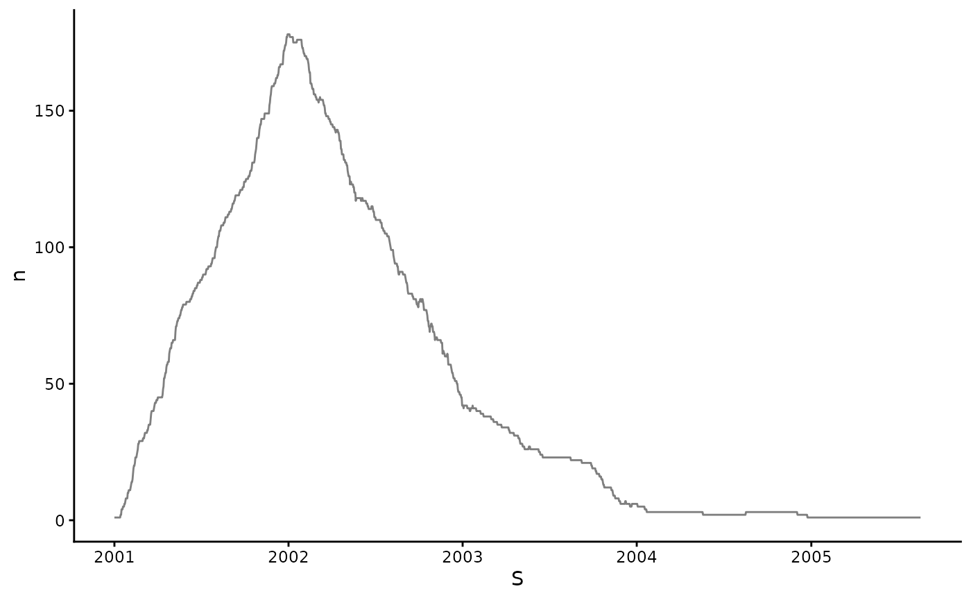

Next, let’s look at the first few rows of observation-level (longitudinal) data:

pander(head(sim_obs_data))

ID	E	O	Y	S	MAA status	Obs ID
1	2001-06-16	2002-06-17	1	2002-03-11	MAA+	1
1	2001-06-16	2002-07-15	0	2002-03-11	MAA-	2
1	2001-06-16	2002-08-12	1	2002-03-11	MAA+	3
1	2001-06-16	2002-09-09	0	2002-03-11	MAA-	4
1	2001-06-16	2002-12-02	0	2002-03-11	MAA-	5
1	2001-06-16	2003-02-24	0	2002-03-11	MAA-	6

O is the observation date
Y is the MAA classification (1 = “recent infection”, 0 = “long-term infection”)

The two tables are linked by the variable ID.

We can visualize the data:

sim_data |> 
plot_censoring_data(
        included_IDs = 1:10,
        labelled_IDs = NULL,
        # xmax = lubridate::ymd("2003-01-01"),
        s_vjust = -1
    ) +
  theme(axis.ticks.y = element_blank())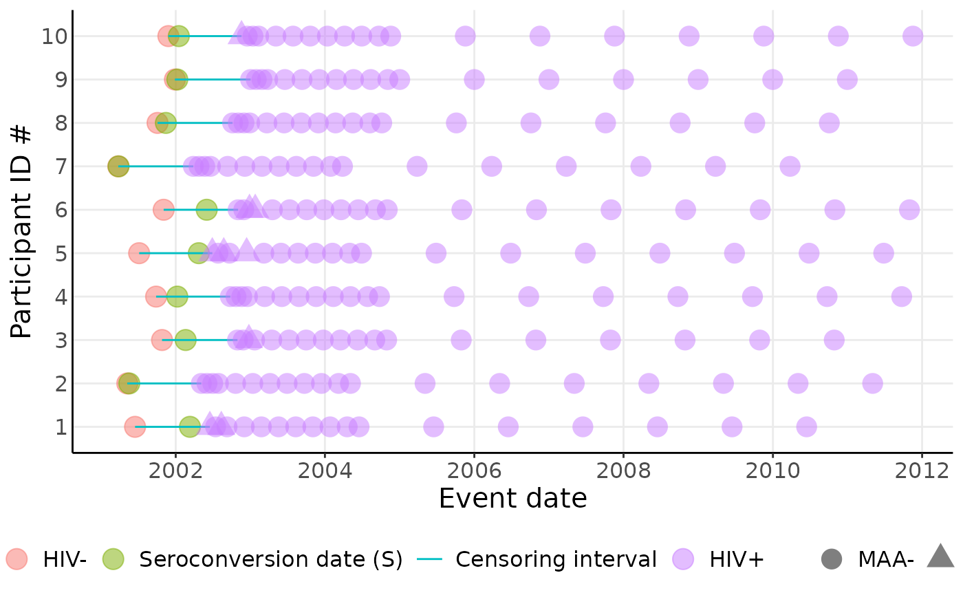

Now, we will apply our proposed analysis (this takes a couple of minutes; use argument verbose = TRUE to print progress messages):

EM_algorithm_outputs = fit_joint_model(
  obs_level_data = sim_obs_data,
  participant_level_data = sim_participant_data,
  bin_width = 7,
  EM_max_iterations = 150,
  verbose = FALSE)

The output of fit_joint_model() is a list with several components:

names(EM_algorithm_outputs)
#> [1] "Theta"               "Mu"                  "Omega"              
#> [4] "converged"           "iterations"          "convergence_metrics"
#> [7] "convergence_stats"

Theta is the vector of estimated logistic regression coefficients for $P(Y|T)$ (intercept and slope):


pander(EM_algorithm_outputs$Theta)

(Intercept)	T
1.019	-3.953

Mu is the corresponding $\hat{\mu}$ estimate:

mu_est_EM = EM_algorithm_outputs$Mu
print(mu_est_EM)
#> [1] 122.5193

Omega is the corresponding $\hat{\omega}(s)$ estimate:

omega_est_EM <- EM_algorithm_outputs$Omega

omega_est_EM |> graph_omega()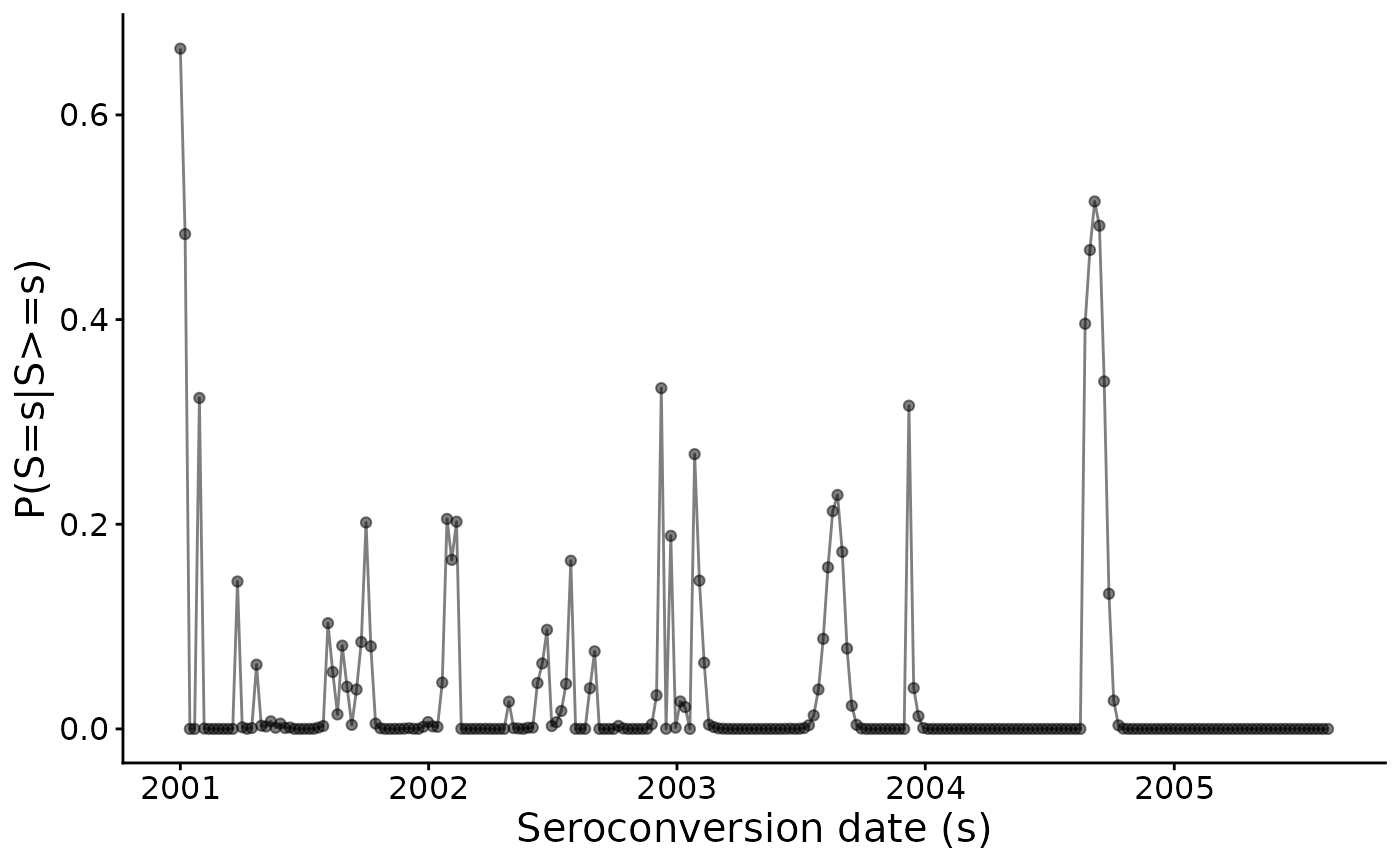

converged indicates whether the algorithm reached its convergence criterion (= 1 if converged, = 0 if not).

EM_algorithm_outputs$converged
#> [1] 1

iterations is the number of EM iterations that the algorithm performed:

EM_algorithm_outputs$iterations
#> [1] 112

convergence_metrics gives the values of all four metrics that we might use to evaluate convergence:

diff logL: change in log-likelihood between iterations
diff mu: change in $\hat{\mu}$
max abs diff coefs: $\max_{j\in 0:1} \{|\hat{\theta}_j^{(k)} - \hat{\theta}_j^{(k-1)}|\}$
max abs rel diff coefs: $\max_{j\in 0:1} \{|(\hat{\theta}_j^{(k)} - \hat{\theta}_j^{(k-1)})/\hat{\theta}_j^{(k-1)}|\}$

By default, the convergence criterion is: diff logL < 0.1 and max abs rel diff coefs < 0.0001.

pander(EM_algorithm_outputs$convergence_metrics)

diff logL	diff mu	max abs diff coefs	max abs rel diff coefs
0.008769	0.008171	0.0001012	9.931e-05

Next, we perform an alternative analysis using midpoint imputation:


theta_est_midpoint = fit_midpoint_model(
  obs_level_data = sim_obs_data,
  participant_level_data = sim_participant_data
)

pander(theta_est_midpoint)

(Intercept)	T_midpoint
0.7572	-3.662

Here, we perform an alternative analysis using uniform imputation:

# uniform imputation:
theta_est_uniform = fit_uniform_model(
  obs_level_data = sim_obs_data,
  participant_level_data = sim_participant_data
)

pander(theta_est_uniform)

theta0	theta1
-0.549	-2.037

Now, let’s graph the results. First, let’s plot the true and estimated CDFs for the distribution of seroconversion date, for individuals who enroll on the first calendar day of the cohort study:


plot1 = plot_CDF(
  true_hazard_alpha = hazard_alpha,
  true_hazard_beta = hazard_beta,
  omega_hat = EM_algorithm_outputs$Omega)

print(plot1)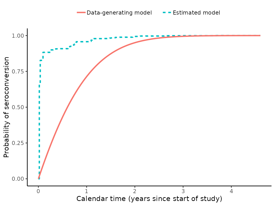

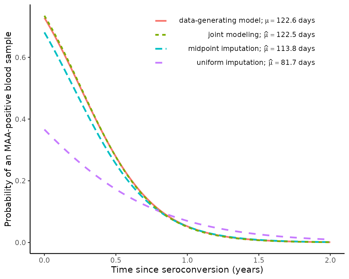
We can see that our joint modeling approach hasn’t estimated this distribution very accurately for this particular simulated dataset. Nevertheless, the next graph will show us that the joint model very accurately estimates the true distribution $P(Y|T)$ and the true value of $\mu$ :


plot2 = plot_phi_curves(
  theta_true = theta_true,
  theta.hat_uniform = theta_est_uniform,
  theta.hat_midpoint = theta_est_midpoint,
  theta.hat_joint = EM_algorithm_outputs$Theta)

print(plot2)