We sketch the argument for the scalar-parameter case (\(\theta\) is scalar and \(H_0: \theta = \theta_0\) imposes one constraint, so \(q = 1\)). For this point null, the restricted MLE is \(\hat\theta_0 = \theta_0\), so \(\ell(\hat\theta_0) = \ell(\theta_0)\) and the LR statistic reduces to \(\Lambda = 2{\left(\ell(\hat\theta_{\text{ML}}) - \ell(\theta_0)\right)}\). The multivariate case follows the same steps in matrix form (see Dobson and Barnett (2018) §5.7 or Wilks (1938) for the full proof).
Step 1: Taylor expansion of \(\ell(\theta_0)\) around \(\hat\theta_{\text{ML}}\).
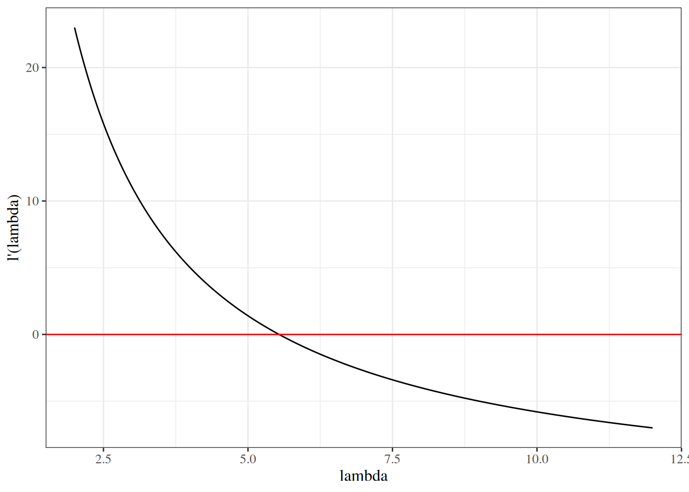
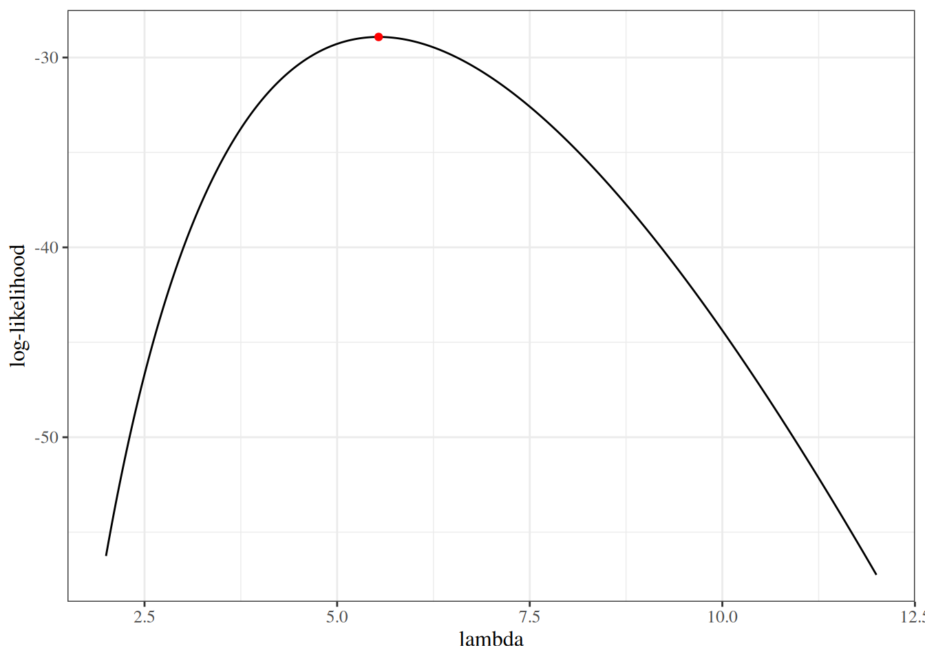
Since \(\hat\theta_{\text{ML}}\) maximizes \(\ell\), the score at \(\hat\theta_{\text{ML}}\) is zero: \[
\ell'(\hat\theta_{\text{ML}}) = 0
\]
Expanding \(\ell(\theta_0)\) around \(\hat\theta_{\text{ML}}\) by Taylor’s theorem: \[
\begin{aligned}
\ell(\theta_0)
&\approx
\ell(\hat\theta_{\text{ML}})
+ \underbrace{\ell'(\hat\theta_{\text{ML}})}_{= \, 0}(\theta_0 - \hat\theta_{\text{ML}})
+ \frac{1}{2}\ell''(\hat\theta_{\text{ML}})(\theta_0 - \hat\theta_{\text{ML}})^2
\end{aligned}
\]
Since the score term vanishes: \[
\begin{aligned}
\ell(\theta_0)
&\approx
\ell(\hat\theta_{\text{ML}})
+ \frac{1}{2}\ell''(\hat\theta_{\text{ML}})(\theta_0 - \hat\theta_{\text{ML}})^2
\end{aligned}
\]
Rearranging: \[
\begin{aligned}
2{\left(\ell(\hat\theta_{\text{ML}}) - \ell(\theta_0)\right)}
&\approx
-\ell''(\hat\theta_{\text{ML}})(\hat\theta_{\text{ML}}- \theta_0)^2
\\&=
{\left(-\ell''(\hat\theta_{\text{ML}})\right)}(\hat\theta_{\text{ML}}- \theta_0)^2
\end{aligned}
\]
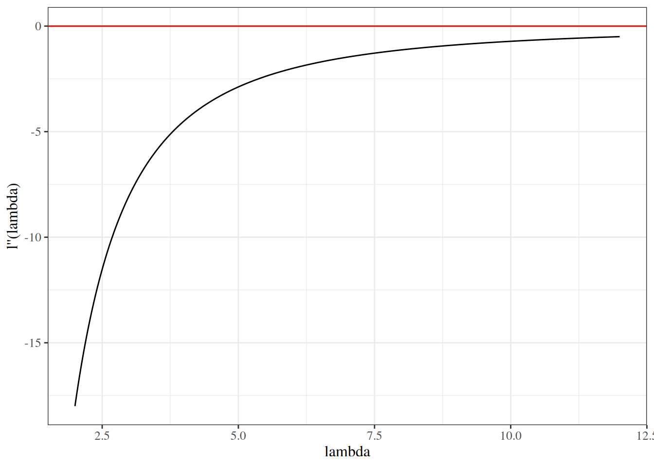
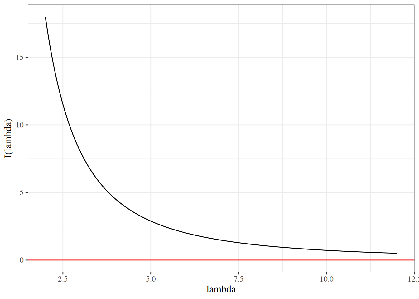
Step 2: Recognizing the observed information.
The negative Hessian is the observed information \(I{\left(\hat\theta_{\text{ML}}\right)} = -\ell''(\hat\theta_{\text{ML}})\). Under regularity conditions, the normalized observed information satisfies \[
\frac{1}{n}I{\left(\hat\theta_{\text{ML}}\right)}
\to
\mathcal{I}(\theta_0),
\] where \(\mathcal{I}(\theta_0)\) is the Fisher information per observation. This uses the law of large numbers together with consistency of \(\hat\theta_{\text{ML}}\), so evaluation at the random point \(\hat\theta_{\text{ML}}\) can be replaced asymptotically by evaluation at \(\theta_0\) via Slutsky’s theorem. Hence \(I{\left(\hat\theta_{\text{ML}}\right)} \approx n \mathcal{I}(\theta_0)\), and therefore \[
\begin{aligned}
2{\left(\ell(\hat\theta_{\text{ML}}) - \ell(\theta_0)\right)}
&\approx
I{\left(\hat\theta_{\text{ML}}\right)} \cdot (\hat\theta_{\text{ML}}- \theta_0)^2
\\&\approx
n \mathcal{I}(\theta_0) \cdot (\hat\theta_{\text{ML}}- \theta_0)^2
\end{aligned}
\]
Step 3: Standardizing to a squared standard normal.
Define the standardized estimation error: \[
z
\stackrel{\text{def}}{=}
\sqrt{n \mathcal{I}(\theta_0)}
\cdot (\hat\theta_{\text{ML}}- \theta_0)
\]
Then: \[
\begin{aligned}
2{\left(\ell(\hat\theta_{\text{ML}}) - \ell(\theta_0)\right)}
&\approx
z^2
\end{aligned}
\]
Step 4: Applying the CLT for MLEs.
By Theorem 6 (the CLT for MLEs): \[
\hat\theta_{\text{ML}}
\ \dot{\sim} \
\text{N}{\left(\theta_0,\; {\left[n\mathcal{I}(\theta_0)\right]}^{-1}\right)}
\]
Therefore: \[
z
= \sqrt{n \mathcal{I}(\theta_0)} \cdot (\hat\theta_{\text{ML}}- \theta_0)
\ \dot{\sim} \
N(0, 1)
\]
and so: \[
\Lambda
=
2{\left(\ell(\hat\theta_{\text{ML}}) - \ell(\theta_0)\right)}
\approx z^2
\overset{d}{\to}
\chi^2_1
\]
Extension to \(q\) constraints.
For the general case of \(q\) constraints (comparing a full model with \(p\) parameters to a restricted model with \(p_0 = p - q\) free parameters), the argument proceeds in matrix form. The LR statistic is a quadratic form in the relevant \(q\)-dimensional component of the score at the restricted MLE, evaluated against the inverse of the observed information matrix. Under \(H_0\), this \(q\)-dimensional component (equivalently, the difference between the unrestricted and restricted estimators in the constrained directions) is approximately multivariate normal with the appropriate covariance structure, so the resulting quadratic form converges in distribution to \(\chi^2_q\).