---
title: "Basic Statistical Methods"
format:
html: default
revealjs:
output-file: basic-statistical-methods-slides.html
pdf:
output-file: basic-statistical-methods-handout.pdf
---
{{< include shared-config.qmd >}}
## Acknowledgements {.unnumbered}
This content is adapted from @vittinghoff2e, Chapter 3.
# Introduction
This appendix reviews fundamental statistical methods
that are prerequisites for the main content of this course.
Most of this material should be familiar from Epi 202 and Epi 203.
---
## Example dataset: HERS {#sec-hers-intro .unnumbered}
Throughout this appendix we use the HERS dataset as a running example.
{{< include _subfiles/shared/_sec_hers_intro.qmd >}}
```{r}
#| eval: false
library(haven)
hers <- haven::read_dta(
  paste0(
    "https://regression.ucsf.edu/sites/g/files",
    "/tkssra6706/f/wysiwyg/home/data/hersdata.dta"
  )
)
```
```{r}
#| include: false
library(haven)
hers <- haven::read_dta(
fs::path_package("rme", "extdata/hersdata.dta")
)
```
# Descriptive Statistics {#sec-descriptive-stats}
See @vittinghoff2e, §3.2.
## Summary statistics for continuous variables {#sec-summary-continuous}
::: {#def-sample-mean}
#### Sample mean
The **sample mean** of $n$ observations $x_1, \ldots, x_n$ is:
$$\bar{x} = \frac{1}{n} \sum_{i=1}^{n} x_i$$
:::
::: {#def-sample-variance}
#### Sample variance
The **sample variance** is:
$$s^2 = \frac{1}{n-1} \sum_{i=1}^{n} (x_i - \bar{x})^2$$
The divisor $n - 1$ (rather than $n$)
makes $s^2$ an [unbiased](estimation.qmd#def-unbiased) estimator
of the population variance $\sigma^2$.
:::
::: {#def-sample-sd}
#### Sample standard deviation
The **sample standard deviation** is $s = \sqrt{s^2}$.
It is expressed in the same units as the original data,
making it more interpretable than the variance.
:::
::: {#def-sample-median}
#### Sample median
The **sample median** is the middle value
when observations are sorted in ascending order.
For $n$ observations:
- If $n$ is odd, the median is the $\frac{n+1}{2}$th order statistic.
- If $n$ is even, the median is the average of the
$\frac{n}{2}$th and $\frac{n}{2}+1$th order statistics.
The median is more robust to outliers than the mean.
:::
::: {#def-IQR}
#### Interquartile range
The **interquartile range (IQR)** is the difference between the 75th percentile
(the third quartile, $Q_3$) and the 25th percentile
(the first quartile, $Q_1$):
$$\text{IQR} = Q_3 - Q_1$$
Like the median, the IQR is robust to outliers.
:::
## Summary statistics for categorical variables {#sec-summary-categorical}
::: {#def-sample-proportion}
#### Sample proportion
For a binary outcome,
the **sample proportion** of "successes" (coded as 1) is:
$$\hat{p} = \frac{k}{n}$$
where $k$ is the number of successes and $n$ is the total sample size.
:::
## Computing summary statistics in R {#sec-summary-R}
The `tbl_summary()` function from the `gtsummary` package
produces formatted summary tables:
::: {#exm-hers-summary}
#### HERS baseline summary statistics
```{r}
#| label: tbl-hers-summary
#| code-fold: false
library(dplyr)
library(gtsummary)
library(haven)

hers |>
  mutate(
    HT = haven::as_factor(HT),
    exercise = haven::as_factor(exercise),
    smoking = haven::as_factor(smoking),
    diabetes = haven::as_factor(diabetes)
  ) |>
  select(age, BMI, glucose, SBP, DBP, HT, exercise, smoking, diabetes) |>
  tbl_summary(
    by = HT,
    statistic = list(
      all_continuous() ~ "{mean} ({sd})",
      all_categorical() ~ "{n} ({p}%)"
    ),
    digits = all_continuous() ~ 1,
    label = list(
      age ~ "Age (years)",
      BMI ~ "BMI (kg/m²)",
      glucose ~ "Fasting glucose (mg/dL)",
      SBP ~ "Systolic BP (mmHg)",
      DBP ~ "Diastolic BP (mmHg)",
      exercise ~ "Exercises regularly",
      smoking ~ "Current smoker",
      diabetes ~ "Diabetes"
    )
  ) |>
  add_overall() |>
  bold_labels()
```
:::
## Exploratory data analysis {#sec-eda}
Graphical summaries reveal aspects of the data distribution
that summary statistics may miss,
such as skewness, multimodality, and outliers.
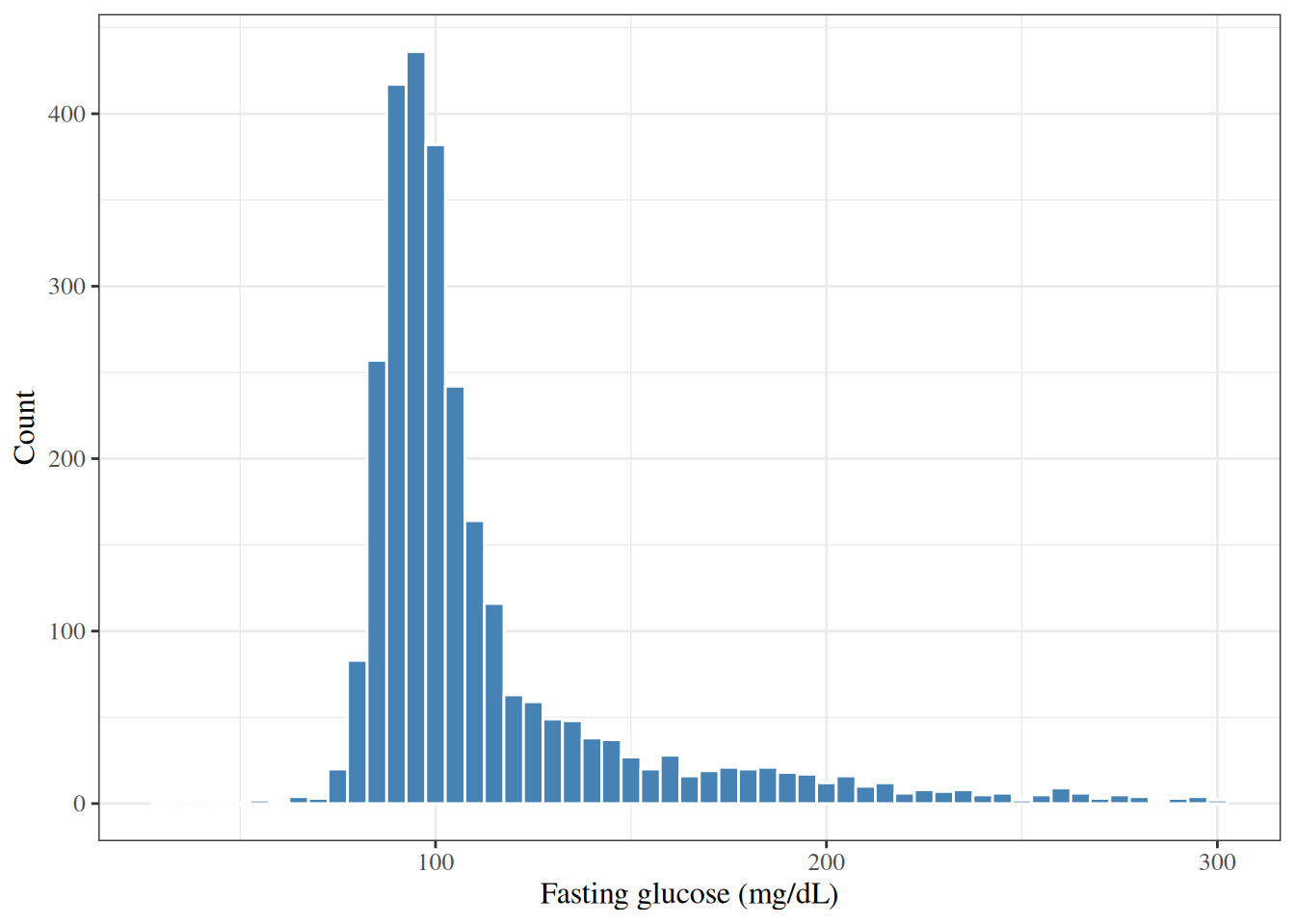
### Histograms {#sec-histograms}
A **histogram** displays the distribution of a continuous variable
by dividing the range of values into intervals (bins)
and plotting the number or proportion of observations in each bin.
::: {#exm-hers-histogram}
#### Distribution of fasting glucose
```{r}
#| label: fig-hers-histogram
#| fig-cap: "Distribution of fasting glucose (mg/dL) in HERS participants"
#| code-fold: false
library(ggplot2)

hers |>
  ggplot() +
  aes(x = glucose) +
  geom_histogram(binwidth = 5, fill = "steelblue", color = "white") +
  labs(
    x = "Fasting glucose (mg/dL)",
    y = "Count"
  )
```
:::
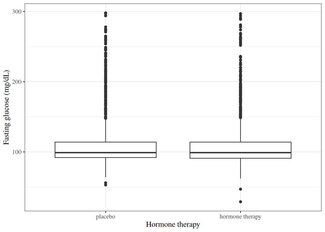
### Boxplots {#sec-boxplots}
A **boxplot** (box-and-whisker plot) summarizes the distribution of a continuous variable
using five statistics:
the minimum, the first quartile ($Q_1$),
the median, the third quartile ($Q_3$), and the maximum
(with outliers plotted separately).
::: {#exm-hers-boxplot}
#### Fasting glucose by hormone therapy group
```{r}
#| label: fig-hers-boxplot
#| fig-cap: "Fasting glucose by hormone therapy assignment in HERS"
#| code-fold: false
hers |>
  mutate(HT = haven::as_factor(HT)) |>
  ggplot() +
  aes(x = HT, y = glucose) +
  geom_boxplot() +
  labs(
    x = "Hormone therapy",
    y = "Fasting glucose (mg/dL)"
  )
```
:::
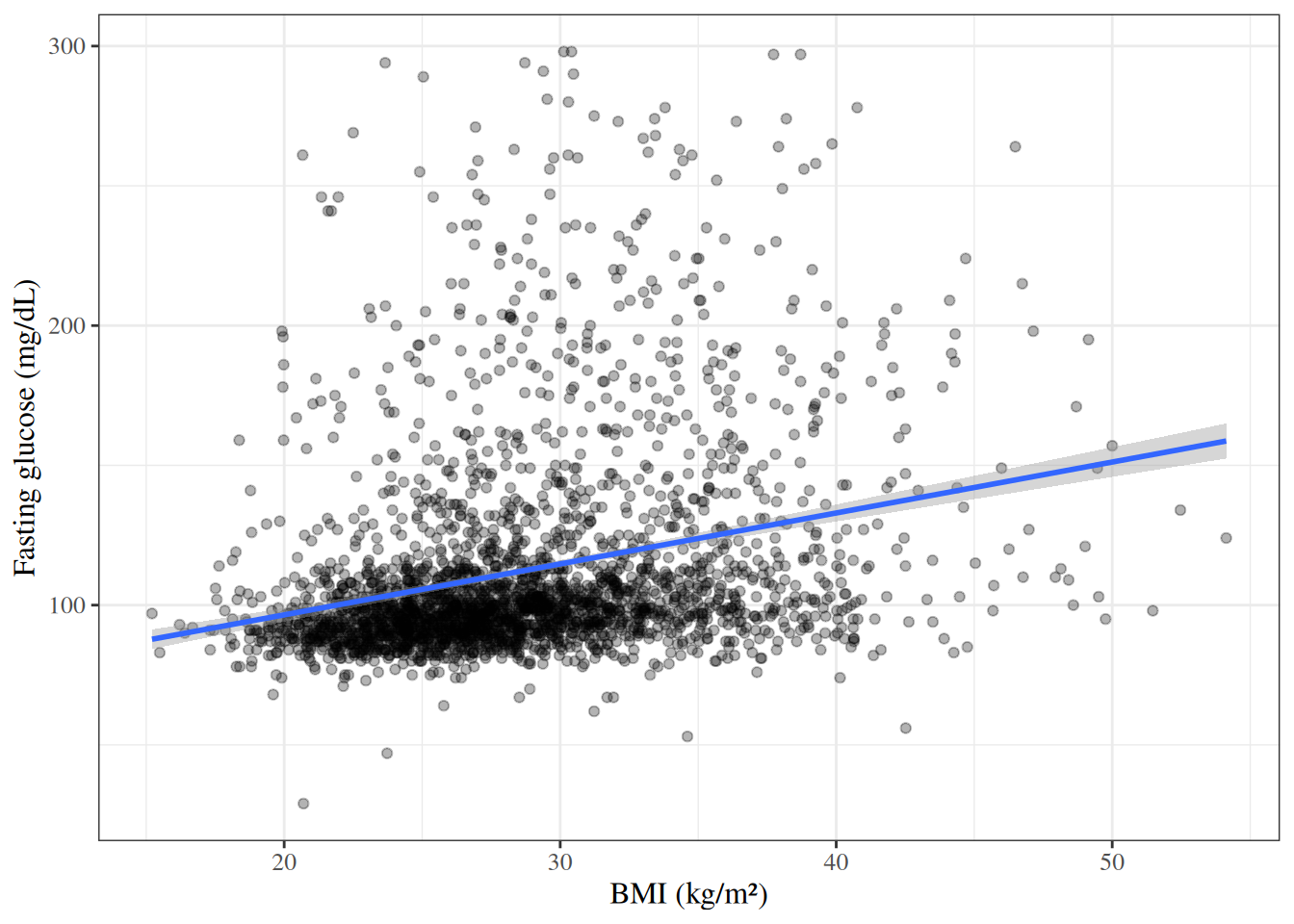
### Scatterplots {#sec-scatterplots}
A **scatterplot** displays the joint distribution of two continuous variables
by plotting each observation as a point.
::: {#exm-hers-scatter}
#### BMI versus fasting glucose
```{r}
#| label: fig-hers-scatter
#| fig-cap: "Fasting glucose versus BMI in HERS participants"
#| code-fold: false
hers |>
  ggplot() +
  aes(x = BMI, y = glucose) +
  geom_point(alpha = 0.3) +
  geom_smooth(method = "lm", se = TRUE) +
  labs(
    x = "BMI (kg/m²)",
    y = "Fasting glucose (mg/dL)"
  )
```
:::
# Comparing Two Groups: Continuous Outcomes {#sec-two-group-continuous}
See @vittinghoff2e, §3.3.
## Hypotheses {#sec-hypotheses}
::: {#def-null-hypothesis}
#### Null hypothesis
The **null hypothesis** $H_0$ is a specific claim
about the population parameter(s) that we test against the data.
In a two-group comparison of means,
the null hypothesis is typically that the two group means are equal:
$$H_0: \mu_1 = \mu_2$$
:::
::: {#def-alternative-hypothesis}
#### Alternative hypothesis
The **alternative hypothesis** $H_1$ (or $H_A$) is the claim
we are trying to find evidence for.
For a two-sided test:
$$H_1: \mu_1 \neq \mu_2$$
:::
## The two-sample t-test {#sec-two-sample-t-test}
::: {#def-two-sample-t-test}
#### Two-sample t-test
The **two-sample t-test** (Welch's t-test)
tests whether the means of two independent groups are equal.
For samples of sizes $n_1$ and $n_2$ from two groups
with sample means $\bar{x}_1$, $\bar{x}_2$
and sample variances $s_1^2$, $s_2^2$,
the test statistic is:
$$t = \frac{\bar{x}_1 - \bar{x}_2}{\sqrt{\dfrac{s_1^2}{n_1} + \dfrac{s_2^2}{n_2}}}$$
Under $H_0$, this statistic follows (approximately) a $t$-distribution
with degrees of freedom estimated by the Welch-Satterthwaite equation.
:::
::: callout-note
#### Welch's t-test vs. pooled t-test
Welch's t-test (the default in R's `t.test()`)
does not assume equal variances across groups.
The pooled t-test assumes equal variances ($\sigma_1^2 = \sigma_2^2$)
and pools the two sample variances into a single estimate.
Welch's t-test is generally preferred
because the equal-variance assumption is rarely verifiable in practice
[@vittinghoff2e §3.3].
:::
::: {#exm-hers-ttest}
#### Comparing fasting glucose between hormone therapy groups
We test $H_0: \mu_\text{placebo} = \mu_\text{HT}$
vs. $H_1: \mu_\text{placebo} \neq \mu_\text{HT}$.
```{r}
#| code-fold: false
glucose_placebo <- hers |> filter(HT == 0) |> pull(glucose)
glucose_HT <- hers |> filter(HT == 1) |> pull(glucose)
t.test(glucose_HT, glucose_placebo)
```
:::
## One-sample t-test {#sec-one-sample-t-test}
::: {#def-one-sample-t-test}
#### One-sample t-test
The **one-sample t-test** tests whether the mean of a single population
equals a specified null value $\mu_0$:
$$H_0: \mu = \mu_0 \qquad H_1: \mu \neq \mu_0$$
The test statistic is:
$$t = \frac{\bar{x} - \mu_0}{s / \sqrt{n}}$$
Under $H_0$, $t \sim t_{n-1}$ (a t-distribution with $n-1$ degrees of freedom).
:::
## Paired t-test {#sec-paired-t-test}
::: {#def-paired-t-test}
#### Paired t-test
The **paired t-test** compares two related measurements
(e.g., pre- and post-treatment values from the same subjects).
Let $d_i = x_{i,1} - x_{i,2}$ be the within-subject difference;
the test reduces to a one-sample t-test on the differences:
$$H_0: \mu_d = 0 \qquad H_1: \mu_d \neq 0$$
:::
::: {#exm-hers-paired}
#### Change in glucose over follow-up
```{r}
#| code-fold: false
# glucose1 is follow-up glucose; glucose is baseline
t.test(hers$glucose1, hers$glucose, paired = TRUE)
```
:::
## Confidence intervals for the difference in means {#sec-CI-diff-means}
A two-sided $(1-\alpha) \cdot 100\%$ confidence interval
for $\mu_1 - \mu_2$ is:
$$(\bar{x}_1 - \bar{x}_2) \pm t^*_{df} \cdot \sqrt{\frac{s_1^2}{n_1} + \frac{s_2^2}{n_2}}$$
where $t^*_{df}$ is the appropriate critical value from the t-distribution.
The confidence interval is returned by `t.test()` in R
alongside the hypothesis test result.
For more on confidence intervals,
see [Statistical Inference](inference.qmd#sec-CI).
# One-Way Analysis of Variance {#sec-anova}
**Analysis of variance (ANOVA)** generalizes the two-sample t-test
to compare means across $k \geq 2$ groups.
::: {#def-one-way-anova}
#### One-way ANOVA
In a **one-way ANOVA**, we test:
$$H_0: \mu_1 = \mu_2 = \cdots = \mu_k$$
vs. the alternative that at least one mean differs.
The F-statistic compares the **between-group variance**
to the **within-group variance**:
$$F = \frac{\text{MS}_\text{between}}{\text{MS}_\text{within}}
= \frac{\text{SS}_\text{between}/(k-1)}{\text{SS}_\text{within}/(n-k)}$$
Under $H_0$, $F \sim F_{k-1, n-k}$.
:::
::: {#exm-hers-anova}
#### Fasting glucose by race/ethnicity
```{r}
#| code-fold: false
aov_result <- aov(glucose ~ factor(raceth), data = hers)
summary(aov_result)
```
:::
::: callout-note
#### ANOVA as a special case of linear regression
One-way ANOVA is equivalent to a linear regression model
with a single categorical predictor.
See [Linear Models Overview](Linear-models-overview.qmd) for details.
:::
# Comparing Two Groups: Categorical Outcomes {#sec-two-group-categorical}
See @vittinghoff2e, §3.5.
## Contingency tables {#sec-contingency-tables}
::: {#def-contingency-table}
#### Contingency table
A **contingency table** (cross-tabulation) displays
the joint frequencies of two categorical variables.
For two binary variables,
this is a $2 \times 2$ table with cells $a$, $b$, $c$, $d$:
| | Outcome = 1 | Outcome = 0 | Total |
|--------------------|:-----------:|:-----------:|:---------:|
| Exposure = 1 | $a$ | $b$ | $a + b$ |
| Exposure = 0 | $c$ | $d$ | $c + d$ |
| Total | $a + c$ | $b + d$ | $n$ |
:::
::: {#exm-hers-crosstab}
#### Exercise by hormone therapy group
```{r}
#| label: tbl-hers-crosstab
#| tbl-cap: "Exercise by hormone therapy group in HERS"
#| code-fold: false
hers |>
  mutate(
    HT = haven::as_factor(HT),
    exercise = haven::as_factor(exercise)
  ) |>
  gtsummary::tbl_cross(
    row = exercise,
    col = HT,
    label = list(
      exercise ~ "Exercises regularly",
      HT ~ "Hormone therapy"
    ),
    percent = "row"
  )
```
:::
## The chi-square test {#sec-chi-square}
::: {#def-chi-square-test}
#### Pearson chi-square test
The **Pearson chi-square test** tests whether two categorical variables are independent.
For a $2 \times 2$ table,
the test statistic is:
$$\chi^2 = \sum_{i,j} \frac{(O_{ij} - E_{ij})^2}{E_{ij}}$$
where $O_{ij}$ is the observed cell count
and $E_{ij} = \frac{(\text{row total}) \times (\text{column total})}{n}$
is the expected cell count under independence.
Under $H_0$ (independence), $\chi^2 \sim \chi^2_1$
for a $2 \times 2$ table.
:::
::: {#exm-hers-chisq}
#### Chi-square test: exercise vs. hormone therapy
```{r}
#| code-fold: false
chisq.test(hers$exercise, hers$HT)
```
:::
## Fisher's exact test {#sec-fisher}
::: {#def-fishers-exact}
#### Fisher's exact test
**Fisher's exact test** computes the exact probability of observing
a $2 \times 2$ table at least as extreme as the observed table,
given the marginal totals and under the null hypothesis of independence.
It is preferred over the chi-square test when cell counts are small
(typically when any expected cell count is less than 5).
:::
::: {#exm-hers-fisher}
#### Fisher's exact test
```{r}
#| code-fold: false
fisher.test(hers$exercise, hers$HT)
```
:::
## Measures of association for 2×2 tables {#sec-2x2-measures}
See [Odds Ratios and Relative Risks](OR-RR.qmd) for definitions and formulas.
# Correlation {#sec-correlation}
See @vittinghoff2e, §3.6.
## Pearson correlation coefficient {#sec-pearson}
::: {#def-pearson-r}
#### Pearson correlation coefficient
The **Pearson correlation coefficient** measures the strength and direction
of the linear association between two continuous variables $X$ and $Y$:
$$r = \frac{\sum_{i=1}^{n} (x_i - \bar{x})(y_i - \bar{y})}
{\sqrt{\sum_{i=1}^{n}(x_i - \bar{x})^2 \sum_{i=1}^{n}(y_i - \bar{y})^2}}$$
$r$ ranges from $-1$ (perfect negative linear relationship) to $+1$
(perfect positive linear relationship);
$r = 0$ indicates no linear association.
:::
::: {#exm-hers-cor}
#### Correlation between BMI and glucose
```{r}
#| code-fold: false
cor.test(hers$BMI, hers$glucose, method = "pearson")
```
:::
## Spearman rank correlation {#sec-spearman}
::: {#def-spearman-r}
#### Spearman rank correlation
The **Spearman rank correlation** $r_S$
is the Pearson correlation computed on the *ranks* of the observations.
It measures the strength and direction of any *monotone* association
(not just linear) and is more robust to outliers.
:::
::: {#exm-hers-spearman}
#### Spearman correlation between BMI and glucose
```{r}
#| code-fold: false
cor.test(hers$BMI, hers$glucose, method = "spearman")
```
:::
# Simple Linear Regression {#sec-simple-linear-regression}
See @vittinghoff2e, §3.6 and [Linear Models Overview](Linear-models-overview.qmd).
## Model specification {#sec-slr-model}
::: {#def-slr}
#### Simple linear regression model
A **simple linear regression** model relates
a continuous outcome $Y$ to a single predictor $X$:
$$Y_i = \b_0 + \b_1 x_i + \varepsilon_i, \qquad \varepsilon_i \overset{\text{iid}}{\sim} \ndist{0, \sigma^2}$$
- $\b_0$ is the **intercept**:
the expected value of $Y$ when $X = 0$.
- $\b_1$ is the **slope**:
the expected change in $Y$ per one-unit increase in $X$.
- $\varepsilon_i$ are independent Gaussian errors with mean 0 and variance $\sigma^2$.
:::
## Ordinary least squares estimation {#sec-ols}
The parameters $\b_0$ and $\b_1$ are estimated
by minimizing the **residual sum of squares (RSS)**:
$$\text{RSS} = \sum_{i=1}^n (y_i - \hat{y}_i)^2
= \sum_{i=1}^n (y_i - \hat\b_0 - \hat\b_1 x_i)^2$$
The closed-form **ordinary least squares (OLS)** estimators are:
$$\hat\b_1 = r \cdot \frac{s_y}{s_x}, \qquad \hat\b_0 = \bar{y} - \hat\b_1 \bar{x}$$
where $r$ is the Pearson correlation and $s_x$, $s_y$ are the sample standard deviations.
## Fitting a simple linear regression in R {#sec-slr-R}
::: {#exm-hers-slr}
#### Glucose on BMI
```{r}
#| label: tbl-hers-slr
#| code-fold: false
slr_fit <- lm(glucose ~ BMI, data = hers)
summary(slr_fit)
```
The estimated slope is
$\hat\b_1 = `r round(coef(slr_fit)[["BMI"]], 2)`$ mg/dL per kg/m²,
meaning fasting glucose increases by approximately
`r round(coef(slr_fit)[["BMI"]], 2)` mg/dL
for each 1 kg/m² increase in BMI.
:::
## The coefficient of determination ($R^2$) {#sec-r-squared}
::: {#def-r-squared}
#### Coefficient of determination
The **coefficient of determination** $R^2$ measures the proportion of the total
variance in $Y$ that is explained by the linear regression on $X$:
$$R^2 = 1 - \frac{\text{RSS}}{\text{TSS}}
= 1 - \frac{\sum_i (y_i - \hat{y}_i)^2}{\sum_i (y_i - \bar{y})^2}$$
$R^2$ ranges from 0 (no linear relationship)
to 1 (perfect linear fit).
For simple linear regression, $R^2 = r^2$.
:::
## Further reading
For a more thorough treatment of linear regression,
see [Linear Models Overview](Linear-models-overview.qmd)
and @vittinghoff2e, Chapters 4 and 9.