Advanced Quarto Article
2026-05-27
1 Overview
This article demonstrates advanced features of Quarto for package documentation. Unlike vignettes, articles are only available on the documentation website and are not included in the package bundle.
2 When to Use Articles vs Vignettes
Vignettes should be used for:
- Core package documentation
- Essential usage examples
- Content that users need offline
Articles are better for:
- Extended tutorials
- Case studies and detailed examples
- Content with large datasets or external dependencies
- Supplementary material
3 Advanced Quarto Features
3.1 Cross-References
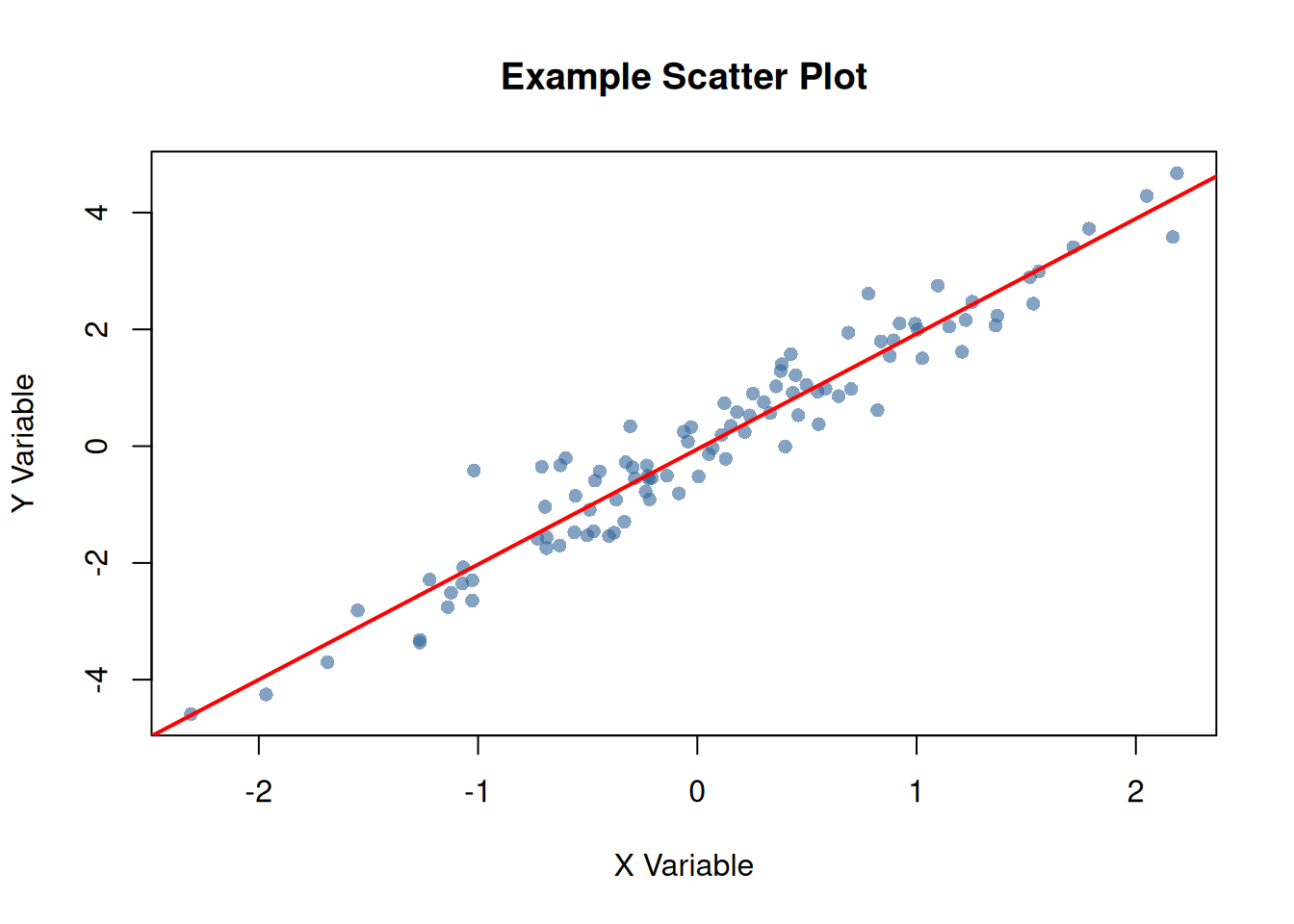
Quarto makes it easy to create cross-references. For example, see Figure 1 for a scatter plot and Table 1 for a summary table.
Code
3.2 Summary Tables
Code
| Statistic | X | Y |
|---|---|---|
| Mean | 0.090 | 0.127 |
| Median | 0.062 | 0.137 |
| SD | 0.913 | 1.865 |
| Min | -2.309 | -4.586 |
| Max | 2.187 | 4.675 |
As shown in Table 1, the variables have similar distributions.
3.3 Code Folding
You can make code chunks foldable:
Show the code for data preparation
# Prepare more complex data
complex_data <- data.frame(
  id = 1:50,
  group = rep(c("A", "B"), each = 25),
  value1 = rnorm(50, 100, 15),
  value2 = rnorm(50, 50, 10)
)

# Calculate group statistics
group_stats <- aggregate(
  cbind(value1, value2) ~ group,
  data = complex_data,
  FUN = function(x) c(mean = mean(x), sd = sd(x))
)

print(group_stats)
#>   group value1.mean value1.sd value2.mean value2.sd
#> 1     A   101.61247  14.63952   51.727220 10.047051
#> 2     B    98.13191  13.84514   53.261796  8.934998
3.4 Tabsets
#>        id              group        value1           value2
#>  Min.   : 1.00   Length   :50   Min.   : 79.60   Min.   :32.43
#>  1st Qu.:13.25   N.unique : 2   1st Qu.: 89.29   1st Qu.:46.76
#>  Median :25.50   N.blank  : 0   Median : 96.64   Median :51.04
#>  Mean   :25.50   Min.nchar: 1   Mean   : 99.87   Mean   :52.49
#>  3rd Qu.:37.75   Max.nchar: 1   3rd Qu.:107.93   3rd Qu.:59.34
#>  Max.   :50.00                  Max.   :132.98   Max.   :72.93
#> id group value1 value2
#> 1 1 A 132.98216 46.24397
#> 2 2 A 119.68619 44.38124
#> 3 3 A 96.02282 46.56083
#> 4 4 A 108.14791 50.90497
#> 5 5 A 93.78490 65.98509
#> 6 6 A 92.85630 49.11435
#> 7 7 A 88.17096 60.80799
#> 8 8 A 91.08074 56.30754
#> 9 9 A 124.76361 48.86360
#> 10 10 A 99.18958 34.670983.5 Advanced Callouts
When using this package in production:
- Always validate input data
- Check for missing values
- Consider computational complexity
Large datasets may require additional memory and processing time.
3.6 Columns Layout
Left Column
This demonstrates a two-column layout in Quarto.
- Feature 1
- Feature 2
- Feature 3
Right Column
You can place different content in each column.
4 Working with Package Functions
Here’s how to use the package’s example function with different inputs:
Code
# Numeric vector
example_function(c(5, 10, 15, 20, 25))
#> [1] 15

# Using with generated data
random_data <- runif(10, min = 0, max = 100)
example_function(random_data)
#> [1] 47.43
5 Theorem Environments
The callouty-theorem extension renders Quarto theorem and proof environments as styled callout blocks. This makes theorems, definitions, examples, and proofs visually distinct and easier to navigate.
5.1 Definitions and Theorems
Proof. See any standard probability textbook.
5.2 Lemmas and Corollaries
5.3 Examples and Exercises
6 Mathematical Notation
Quarto excels at mathematical notation. Here’s an example of a statistical formula:
The standard error of the mean is calculated as:
\[ SE = \frac{s}{\sqrt{n}} \]
where \(s\) is the sample standard deviation and \(n\) is the sample size.
For a confidence interval:
\[ CI = \bar{x} \pm t_{\alpha/2, n-1} \cdot SE \]
7 Tips and Best Practices
Click to expand this section for additional tips:
- Use descriptive chunk labels for better organization
- Set global chunk options at the beginning
- Use cross-references to link related content
- Leverage callouts for important information
- Consider code folding for long code blocks
8 Conclusion
This article demonstrates the advanced capabilities of Quarto for creating rich, interactive documentation for R packages.
9 Learn More
- Visit the package website
- Check out the GitHub repository
- Read the Quarto documentation