---
title: "Probability"
format:
html: default
revealjs:
output-file: probability-slides.html
pdf:
output-file: probability-handout.pdf
---
{{< include shared-config.qmd >}}
---
Most of the content in this chapter should be review from UC Davis Epi 202.
# Core properties of probabilities
## Defining probabilities
:::{#def-probability}
### Probability measure
A **probability measure**, often denoted $\Pr()$ or $\P()$,
is a function whose domain is a
[$\sigma$-algebra](https://en.wikipedia.org/wiki/%CE%A3-algebra)
of possible outcomes, $\mathscr{S}$,
and which satisfies the following properties:
1. For any statistical event $A \in \mathscr{S}$, $\Pr(A) \ge 0$.
2. The probability of the union of all outcomes ($\Omega \eqdef \cup \mathscr{S}$)
is 1:
$$\Pr(\Omega) = 1$$
3. The probability of the union of countably many mutually disjoint events
$A_1, A_2, \ldots$ (where $A_i \cap A_j = \emptyset$ for all $i \neq j$)
is equal to the sum of their probabilities
(*countable additivity* or *sigma-additivity*):
$$\Pr\!\left(\bigcup_{i=1}^{\infty} A_i\right) = \sum_{i=1}^{\infty} \Pr(A_i)$$
:::
::: notes
Property 3 (*countable additivity*) is stronger than *finite additivity*,
which only requires
$$\Pr(A_1 \cup \cdots \cup A_n) = \sum_{i=1}^{n} \Pr(A_i)$$
for every finite collection of mutually disjoint events.
Countable additivity implies finite additivity
(set $A_{n+1} = A_{n+2} = \cdots = \emptyset$ in property 3,
using $\Pr(\emptyset) = 0$),
but not vice versa:
there exist set functions that satisfy finite additivity
but fail countable additivity
(see [Wikipedia: Sigma-additive set function — An additive function which is not σ-additive](https://en.wikipedia.org/wiki/Sigma-additive_set_function#An_additive_function_which_is_not_%CF%83-additive)).
Requiring countable additivity enables results such as
the continuity of probability
(if $A_1 \supseteq A_2 \supseteq \cdots$ with $\bigcap_i A_i = \emptyset$,
then $\Pr(A_i) \to 0$)
and underpins the @thm-total-prob for countable partitions.
:::
---
:::{#thm-prob-subset}
If $A$ and $B$ are statistical events and $A\subseteq B$, then $\Pr(A \cap B) = \Pr(A)$.
:::
---
::: proof
Left to the reader for now.
:::
---
:::{#thm-total-prob-1}
$$\Pr(A) + \Pr(\neg A) = 1$$
:::
---
::: proof
By properties 2 and 3 of @def-probability.
:::
---
:::{#cor-p-neg0}
$$\Pr(\neg A) = 1 - \Pr(A)$$
:::
---
::: proof
By @thm-total-prob-1 and algebra.
:::
---
:::{#cor-p-neg}
If the probability of an outcome $A$ is $\Pr(A)=\pi$,
then the probability that $A$ does not occur is:
$$\Pr(\neg A)= 1 - \pi$$
:::
---
::: proof
Using @cor-p-neg0:
$$
\ba
\Pr(\neg A) &= 1 - \Pr(A)
\\ &= 1 - \pi
\ea
$$
:::
---
## Conditional probability
:::{#def-conditional-prob}
### Conditional probability
For two events $A$ and $B$ with $\Pr(B) > 0$,
the **conditional probability** of $A$ given $B$,
denoted $\Pr(A \mid B)$,
is:
$$\Pr(A \mid B) \eqdef \frac{\Pr(A \cap B)}{\Pr(B)}$$
:::
---
:::{#thm-law-conditional-prob}
### Law of conditional probability
For any two events $A$ and $B$ with $\Pr(B) > 0$:
$$\Pr(A \cap B) = \Pr(A \mid B) \cd \Pr(B)$$
:::
---
::: proof
Rearranging @def-conditional-prob:
$$
\ba
\Pr(A \mid B) &= \frac{\Pr(A \cap B)}{\Pr(B)}
\\ \Pr(A \cap B) &= \Pr(A \mid B) \cd \Pr(B)
\ea
$$
:::
---
:::{#exm-law-conditional-prob}
#### Applying the law of conditional probability
Suppose 30% of adults exercise regularly ($\Pr(E) = 0.30$),
and among adults who exercise regularly,
60% have low blood pressure ($\Pr(L \mid E) = 0.60$).
Then the probability that a randomly selected adult both exercises
regularly and has low blood pressure is:
$$
\ba
\Pr(L \cap E) &= \Pr(L \mid E) \cd \Pr(E)
\\&= 0.60 \cd 0.30
\\&= 0.18
\ea
$$
:::
---
:::{#thm-total-prob}
### Law of total probability
If $B_1, B_2, \ldots$ is a countable partition of the sample space
(i.e., countably many mutually exclusive events whose union is the entire sample space),
then for any event $A$:
$$\Pr(A) = \sum_{i=1}^{\infty} \Pr(A \mid B_i) \cd \Pr(B_i)$$
:::
---
::: proof
Since $B_1, B_2, \ldots$ partition the sample space,
the events $A \cap B_1, A \cap B_2, \ldots$ are mutually exclusive and their
union is $A$.
By property 3 of @def-probability (countable additivity),
and then by @thm-law-conditional-prob:
$$
\ba
\Pr(A)
&= \sum_{i=1}^{\infty} \Pr(A \cap B_i)
\\&= \sum_{i=1}^{\infty} \Pr(A \mid B_i) \cd \Pr(B_i)
\ea
$$
:::
---
:::{#thm-bayes}
### Bayes' theorem
For any two events $A$ and $B$ with $\Pr(A) > 0$ and $\Pr(B) > 0$:
$$\Pr(A \mid B) = \frac{\Pr(B \mid A) \cd \Pr(A)}{\Pr(B)}$$
:::
---
::: proof
Apply @def-conditional-prob to both $\Pr(A \mid B)$ and $\Pr(B \mid A)$:
$$
\ba
\Pr(A \mid B)
&= \frac{\Pr(A \cap B)}{\Pr(B)}
\\&= \frac{\Pr(B \mid A) \cd \Pr(A)}{\Pr(B)}
\ea
$$
The second equality follows from @thm-law-conditional-prob applied to $\Pr(B \cap A) = \Pr(B \mid A) \cd \Pr(A)$.
:::
---
:::{#exm-bayes}
#### Positive predictive value of a medical test
Suppose a disease test has 99% sensitivity and 99% specificity,
and the prevalence of the disease in the population is 7%.
Let $D$ be the event "person has the disease"
and $+$ be the event "test is positive".
Then:
- $\Pr(+ \mid D) = 0.99$ (sensitivity)
- $\Pr(\neg + \mid \neg D) = 0.99$ (specificity),
so the false positive rate is $\Pr(+ \mid \neg D) = 1 - 0.99 = 0.01$
- $\Pr(D) = 0.07$ (prevalence)
By Bayes' theorem (@thm-bayes) and the law of total probability (@thm-total-prob):
$$
\ba
\Pr(D \mid +)
&= \frac{\Pr(+ \mid D) \cd \Pr(D)}{\Pr(+)}
\\&= \frac{\Pr(+ \mid D) \cd \Pr(D)}{\Pr(+ \mid D) \cd \Pr(D) + \Pr(+ \mid \neg D) \cd \Pr(\neg D)}
\\&= \frac{0.99 \cd 0.07}{0.99 \cd 0.07 + 0.01 \cd 0.93}
\\&= \frac{0.0693}{0.0693 + 0.0093}
\\&= \frac{0.0693}{0.0786}
\\&\approx 0.88
\ea
$$
Even with a highly accurate test (99% sensitive and 99% specific),
only about 88% of people who test positive actually have the disease,
because the disease prevalence is relatively low (7%).
:::
# Random variables
## Binary variables {#sec-binary-vars}
{{< include binary-vars.qmd >}}
---
## Count variables {#sec-count-vars}
{{< include count-vars.qmd >}}
---
# Key probability distributions
---
{{< include _sec_distn_uses.qmd >}}
## The Bernoulli distribution {#sec-bern-dist}
{{< include bernoulli.qmd >}}
---
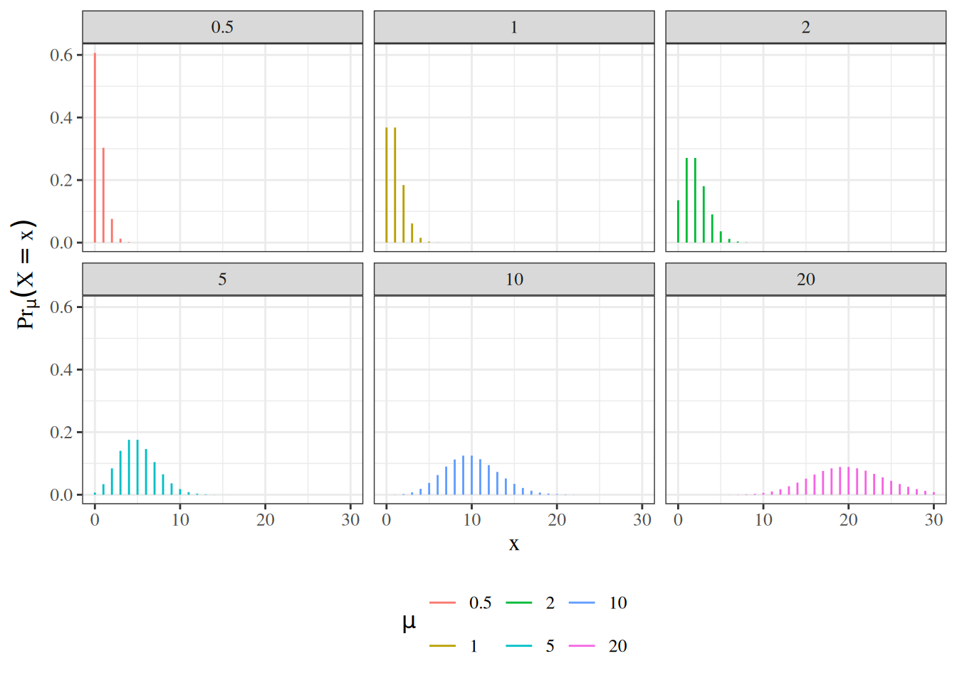
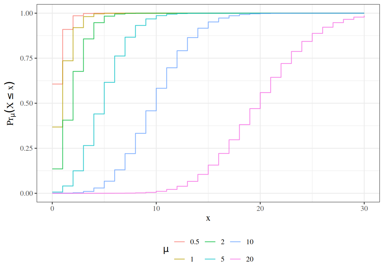
## The Poisson distribution {#sec-poisson-dist}
{{< include poisson.qmd >}}
---
## The Negative-Binomial distribution {#sec-nb-dist}
{{< include negbinom.qmd >}}
## Weibull Distribution {#sec-weibull}
$$
\begin{aligned}
p(t)&= \alpha\lambda x^{\alpha-1}\text{e}^{-\lambda x^\alpha}\\
\haz(t)&=\alpha\lambda x^{\alpha-1}\\
\surv(t)&=\text{e}^{-\lambda x^\alpha}\\
E(T)&= \Gamma(1+1/\alpha)\cdot \lambda^{-1/\alpha}
\end{aligned}
$$
When $\alpha=1$ this is the exponential. When $\alpha>1$ the hazard is
increasing and when $\alpha < 1$ the hazard is decreasing. This provides
more flexibility than the exponential.
We will see more of this distribution later.
# Characteristics of probability distributions
## Probability density function {#sec-prob-dens}
{{< include _def-pdf.qmd >}}
---
:::{#thm-density-vs-CDF}
## Density function is derivative of CDF
The density function $f(t)$ or $\p(T=t)$ for a random variable $T$ at value $t$ is equal to the derivative of the cumulative probability function $F(t) \eqdef P(T\le t)$; that is:
$$f(t) \eqdef \deriv{t} F(t)$$
:::
---
:::{#thm-density-sums-to-one}
### Density functions integrate to 1
For any density function $f(x)$,
$$\int_{x \in \rangef{X}} f(x) dx = 1$$
:::
---
## Hazard function {#sec-prob-haz}
{{< include _def-hazard.qmd >}}
---
{{< include _sec-survival-dist-fns.qmd >}}
---
{{< include _surv_diagram.qmd >}}
---
## Expectation {#sec-expectation}
:::{#def-expectation}
## Expectation, expected value, population mean \index{expectation} \index{expected value}
The **expectation**, **expected value**, or **population mean** of a *continuous* random variable $X$, denoted $\E{X}$, $\mu(X)$, or $\mu_X$, is the weighted mean of $X$'s possible values, weighted by the probability density function of those values:
$$\E{X} = \int_{x\in \rangef{X}} x \cdot \p(X=x)dx$$
The **expectation**, **expected value**, or **population mean** of a *discrete* random variable $X$,
denoted $\E{X}$, $\mu(X)$, or $\mu_X$,
is the mean of $X$'s possible values,
weighted by the probability mass function of those values:
$$\E{X} = \sum_{x \in \rangef{X}} x \cdot \P(X=x)$$
(c.f. <https://en.wikipedia.org/wiki/Expected_value>)
:::
---
:::{#thm-bernoulli-mean}
### Expectation of the Bernoulli distribution
The expectation of a Bernoulli random variable with parameter $\pi$ is:
$$\E{X} = \pi$$
:::
---
:::{.proof}
$$
\ba
\E{X}
&= \sum_{x\in \rangef{X}} x \cd \P(X=x)
\\&= \sum_{x\in \set{0,1}} x \cd \P(X=x)
\\&= \paren{0 \cd \P(X=0)} + \paren{1 \cd \P(X=1)}
\\&= \paren{0 \cd (1-\pi)} + \paren{1 \cd \pi}
\\&= 0 + \pi
\\&= \pi
\ea
$$
:::
---
{{< include _thm-surv-mean.qmd >}}
---
:::{#thm-lotus}
### Law of the Unconscious Statistician (LOTUS)
For any function $g$ of a *discrete* random variable $X$:
$$\E{g(X)} = \sum_{x \in \rangef{X}} g(x) \cd \P(X=x)$$
:::
---
::: proof
Let $Y = g(X)$.
By @def-expectation applied to $Y$:
$$
\ba
\E{g(X)}
&= \E{Y}
\\&= \sum_{y \in \rangef{Y}} y \cd \P(Y=y)
\\&= \sum_{y \in \rangef{Y}} y \cd \P(g(X)=y)
\\&= \sum_{y \in \rangef{Y}} y \cd \sum_{\substack{x \in \rangef{X} \\ g(x) = y}} \P(X=x)
\\&= \sum_{x \in \rangef{X}} g(x) \cd \P(X=x)
\ea
$$
where the last equality follows by rearranging the double sum,
grouping each term $x$ by its image $y = g(x)$.
:::
---
::: notes
LOTUS says that to compute $\E{g(X)}$,
we do not need to first find the distribution of $g(X)$;
we can compute the expectation directly using the distribution of $X$.
For a *continuous* random variable $X$ with density $\p(X=x)$,
the analogous formula is:
$$\E{g(X)} = \int_{x \in \rangef{X}} g(x) \cd \p(X=x)\, dx$$
:::
---
:::{#exm-lotus}
#### Expected value of $X^2$ for a Bernoulli variable
Let $X \sim \Ber(\pi)$.
By LOTUS (@thm-lotus):
$$
\ba
\E{X^2}
&= \sum_{x \in \set{0,1}} x^2 \cd \P(X=x)
\\&= 0^2 \cd \P(X=0) + 1^2 \cd \P(X=1)
\\&= 0^2 \cd (1-\pi) + 1^2 \cd \pi
\\&= 0 + \pi
\\&= \pi
\ea
$$
:::
---
:::{#def-cond-expectation}
### Conditional expectation
**Discrete case.**
Let $X$ and $Y$ be jointly distributed discrete random variables.
The **conditional probability mass function** of $Y$ given $X = x$
(for values of $x$ with $\P(X = x) > 0$) is:
$$\P(Y = y \mid X = x) \eqdef \frac{\P(X = x,\, Y = y)}{\P(X = x)}$$
The **conditional expectation** of $Y$ given $X = x$ is:
$$\E{Y \mid X = x} \eqdef \sum_{y \in \rangef{Y}} y \cd \P(Y = y \mid X = x)$$
**Continuous case.**
Let $X$ and $Y$ be jointly distributed continuous random variables
with joint density $\p(X = x,\, Y = y)$ and marginal density $\p(X = x)$.
The **conditional probability density function** of $Y$ given $X = x$
(for values of $x$ with $\p(X = x) > 0$) is:
$$\p(Y = y \mid X = x) \eqdef \frac{\p(X = x,\, Y = y)}{\p(X = x)}$$
The **conditional expectation** of $Y$ given $X = x$ is:
$$\E{Y \mid X = x} \eqdef \int_{y \in \rangef{Y}} y \cd \p(Y = y \mid X = x)\, dy$$
**Conditional expectation function.**
The **conditional expectation function** $\E{Y \mid X}$ is the function
(and hence random variable) of $X$ obtained by evaluating
$\E{Y \mid X = x}$ at $X$; that is,
$\E{Y \mid X} = g(X)$ where $g(x) \eqdef \E{Y \mid X = x}$.
:::
---
:::{#thm-lie}
### Law of iterated expectations
For any two random variables $X$ and $Y$:
$$\E{Y} = \E{\E{Y \mid X}}$$
:::
---
::: proof
**Discrete case.**
When $X$ and $Y$ are discrete,
applying @def-expectation to $\E{\E{Y \mid X}}$
and then the law of total probability (@thm-total-prob)
applied to the countable partition $\{X = x : x \in \rangef{X}\}$:
$$
\ba
\E{\E{Y \mid X}}
&= \sum_{x \in \rangef{X}} \E{Y \mid X=x} \cd \P(X=x)
\\&= \sum_{x \in \rangef{X}} \paren{\sum_{y \in \rangef{Y}} y \cd \P(Y=y \mid X=x)} \cd \P(X=x)
\\&= \sum_{y \in \rangef{Y}} y \cd \sum_{x \in \rangef{X}} \P(Y=y \mid X=x) \cd \P(X=x)
\\&= \sum_{y \in \rangef{Y}} y \cd \P(Y=y)
\\&= \E{Y}
\ea
$$
**Continuous case.**
When $X$ and $Y$ are continuous,
applying @def-expectation to $\E{\E{Y \mid X}}$
and then using @def-cond-expectation for $\E{Y \mid X=x}$:
$$
\ba
\E{\E{Y \mid X}}
&= \int_{x \in \rangef{X}} \E{Y \mid X=x} \cd \p(X=x)\, dx
\\&= \int_{x \in \rangef{X}} \paren{\int_{y \in \rangef{Y}} y \cd \p(Y=y \mid X=x)\, dy} \cd \p(X=x)\, dx
\\&= \int_{y \in \rangef{Y}} y \cd \paren{\int_{x \in \rangef{X}} \p(Y=y \mid X=x) \cd \p(X=x)\, dx}\, dy
\\&= \int_{y \in \rangef{Y}} y \cd \p(Y=y)\, dy
\\&= \E{Y}
\ea
$$
where the third equality exchanges the order of integration by Fubini's theorem,
and the fourth equality uses
$\int_{x} \p(Y=y \mid X=x) \cd \p(X=x)\, dx = \int_{x} \p(X=x, Y=y)\, dx = \p(Y=y)$
(marginalization of the joint density).
:::
---
:::{#exm-lie}
#### Marginal expectation from conditional expectations
Suppose $X$ is a binary random variable indicating treatment assignment ($X=1$ treated, $X=0$ control),
with $\P(X=1) = 0.5$,
and suppose the outcome $Y$ has conditional expectations:
$$\E{Y \mid X=1} = 10, \quad \E{Y \mid X=0} = 6$$
By the law of iterated expectations (@thm-lie):
$$
\ba
\E{Y}
&= \E{\E{Y \mid X}}
\\&= \E{Y \mid X=1} \cd \P(X=1) + \E{Y \mid X=0} \cd \P(X=0)
\\&= 10 \cd 0.5 + 6 \cd 0.5
\\&= 5 + 3
\\&= 8
\ea
$$
:::
---
{{< include _def-expectation-matrix.qmd >}}
---
## Variance and related characteristics
:::{#def-variance}
### Variance
The variance of a random variable $X$ is the expectation of the squared difference between $X$ and $\E{X}$; that is:
$$
\Var{X} \eqdef \E{(X-\E{X})^2}
$$
:::
---
:::{#thm-variance}
### Simplified expression for variance
$$\Var{X}=\E{X^2} - \sqf{\E{X}}$$
---
::::{.proof}
By linearity of expectation, we have:
$$
\begin{aligned}
\Var{X}
&\eqdef \E{(X-\E{X})^2}\\
&=\E{X^2 - 2X\E{X} + \sqf{\E{X}}}\\
&=\E{X^2} - \E{2X\E{X}} + \E{\sqf{\E{X}}}\\
&=\E{X^2} - 2\E{X}\E{X} + \sqf{\E{X}}\\
&=\E{X^2} - \sqf{\E{X}}\\
\end{aligned}
$$
::::
:::
---
::: {#def-precision}
### Precision
The **precision** of a random variable $X$, often denoted $\tau(X)$, $\tau_X$, or shorthanded as $\tau$, is
the inverse of that random variable's variance; that is:
$$\tau(X) \eqdef \inv{\Var{X}}$$
:::
::: {#def-sd}
### Standard deviation
The standard deviation of a random variable $X$ is the square-root of the variance of $X$:
$$\SD{X} \eqdef \sqrt{\Var{X}}$$
:::
---
:::{#def-cov}
### Covariance
For any two one-dimensional random variables, $X,Y$:
$$\Cov{X,Y} \eqdef \Expf{(X - \E X)(Y - \E Y)}$$
:::
---
:::{#thm-alt-cov}
$$\Cov{X,Y}= \E{XY} - \E{X} \E{Y}$$
:::
---
:::{.proof}
Left to the reader.
:::
---
:::{#lem-cov-xx}
#### The covariance of a variable with itself is its variance
For any random variable $X$:
$$\Cov{X,X} = \Var{X}$$
:::
:::{.proof}
$$
\ba
\Cov{X,X} &= E[XX] - E[X]E[X]
\\ &= E[X^2]-(E[X])^2
\\ &= \Var{X}
\ea
$$
:::
---
{{< include _def-cov-vec-x.qmd >}}
---
{{< include _thm-vcov-elements.qmd >}}
---
:::{#thm-vcov-vec}
### Alternate expression for variance of a random vector
$$
\ba
\Varf{\vX}
&= \Expf{\vX \tp{\vX}} - \paren{\Expp\vX} \tp{\paren{\Expp\vX}}
\ea
$$
:::
---
:::{.proof}
$$
\ba
\Varf{\vX}
&= \Expf{
\paren{\vX - \Expp\vX}
\tp{\paren{\vX - \Expp\vX}}
}
\\
&= \Expf{
\vX \tp{\vX}
- \vX \tp{\paren{\Expp\vX}}
- \paren{\Expp\vX} \tp{\vX}
+ \paren{\Expp\vX} \tp{\paren{\Expp\vX}}
}
\\
&= \Expf{\vX \tp{\vX}}
- \paren{\Expp\vX} \tp{\paren{\Expp\vX}}
- \paren{\Expp\vX} \tp{\paren{\Expp\vX}}
+ \paren{\Expp\vX} \tp{\paren{\Expp\vX}}
\\
&= \Expf{\vX \tp{\vX}}
- \paren{\Expp\vX} \tp{\paren{\Expp\vX}}
\ea
$$
:::
---
{{< include _thm-var-lincom.qmd >}}
---
:::{.proof}
Left to the reader...
:::
---
:::{#cor-var-lincom2}
For any two random variables $X$ and $Y$ and scalars $a$ and $b$:
$$\Var{aX + bY} = a^2 \Var{X} + b^2 \Var{Y} + 2(a \cd b) \Cov{X,Y}$$
:::
---
:::{.proof}
Apply @thm-var-lincom with $n=2$, $X_1 = X$, and $X_2 = Y$.
Or, see <https://statproofbook.github.io/P/var-lincomb.html>
:::
---
:::{#def-homosked}
## homoskedastic, heteroskedastic
A random variable $Y$ is **homoskedastic** (with respect to covariates $X$) if the variance of $Y$ does not vary with $X$:
$$\Varr(Y|X=x) = \ss, \forall x$$
Otherwise it is **heteroskedastic**.
:::
---
:::{#def-indpt}
## Statistical independence
A set of random variables $\X1n$ are **statistically independent**
if their joint probability is equal to the product of their marginal probabilities:
$$\Pr(\Xx1n) = \prodi1n{\Pr(X_i=x_i)}$$
:::
::: notes
::::{.callout-tip}
The symbol for independence, $\ind$, is essentially just $\prod$ upside-down.
So the symbol can remind you of its definition (@def-indpt).
::::
:::
---
:::{#def-cind}
## Conditional independence
A set of random variables $\dsn{Y}$ are **conditionally statistically independent**
given a set of covariates $\X1n$
if the joint probability of the $Y_i$s given the $X_i$s is equal to
the product of their marginal probabilities:
$$\Pr(\dsvn{Y}{y}|\dsvn{X}{x}) = \prodi1n{\Pr(Y_i=y_i|X_i=x_i)}$$
:::
---
:::{#def-ident}
### Identically distributed
A set of random variables $\X1n$ are **identically distributed**
if they have the same range $\rangef{X}$ and if
their marginal distributions $\P(X_1=x_1), ..., \P(X_n=x_n)$ are all
equal to some shared distribution $\P(X=x)$:
$$
\forall i\in \set{1:n}, \forall x \in \rangef{X}: \P(X_i=x) = \P(X=x)
$$
:::
---
:::{#def-cident}
### Conditionally identically distributed
A set of random variables $\dsn{Y}$ are **conditionally identically distributed**
given a set of covariates $\X1n$
if $\dsn{Y}$ have the same range $\rangef{X}$ and if
the distributions $\P(Y_i=y_i|X_i =x_i)$ are all
equal to the same distribution $\P(Y=y|X=x)$:
$$
\P(Y_i=y|X_i=x) = \P(Y=y|X=x)
$$
:::
---
:::{#def-iid}
### Independent and identically distributed
A set of random variables $\dsn{X}$ are **independent and identically distributed**
(shorthand: "$X_i\ \iid$") if they are statistically independent and identically distributed.
:::
---
:::{#def-iid}
### Conditionally independent and identically distributed
A set of random variables $\dsn{Y}$ are **conditionally independent and identically distributed** (shorthand: "$Y_i | X_i\ \ciid$" or just "$Y_i |X_i\ \iid$") given a set of covariates $\dsn{X}$
if $\dsn{Y}$ are conditionally independent given $\dsn{X}$ and $\dsn{Y}$ are identically distributed given
$\dsn{X}$.
:::
{{< include sec-CLT.qmd >}}
# Additional resources
- @problifesaver