Models for Binary Outcomes

Logistic regression and variations

Configuring R

Functions from these packages will be used throughout this document:

library(conflicted) # check for conflicting function definitions
# library(printr) # inserts help-file output into markdown output
library(rmarkdown) # Convert R Markdown documents into a variety of formats.
library(pander) # format tables for markdown
library(ggplot2) # graphics
library(ggfortify) # help with graphics
library(dplyr) # manipulate data
library(tibble) # `tibble`s extend `data.frame`s
library(magrittr) # `%>%` and other additional piping tools
library(haven) # import Stata files
library(knitr) # format R output for markdown
library(tidyr) # Tools to help to create tidy data
library(plotly) # interactive graphics
library(dobson) # datasets from Dobson and Barnett 2018
library(parameters) # format model output tables for markdown
library(haven) # import Stata files
library(latex2exp) # use LaTeX in R code (for figures and tables)
library(fs) # filesystem path manipulations
library(survival) # survival analysis
library(survminer) # survival analysis graphics
library(KMsurv) # datasets from Klein and Moeschberger
library(parameters) # format model output tables for
library(webshot2) # convert interactive content to static for pdf
library(forcats) # functions for categorical variables ("factors")
library(stringr) # functions for dealing with strings
library(lubridate) # functions for dealing with dates and times
library(broom) # Summarizes key information about statistical objects in tidy tibbles
library(broom.helpers) # Provides suite of functions to work with regression model 'broom::tidy()' tibbles

Here are some R settings I use in this document:

rm(list = ls()) # delete any data that's already loaded into R

conflicts_prefer(dplyr::filter)
ggplot2::theme_set(
  ggplot2::theme_bw() + 
        # ggplot2::labs(col = "") +
    ggplot2::theme(
      legend.position = "bottom",
      text = ggplot2::element_text(size = 12, family = "serif")))

knitr::opts_chunk$set(message = FALSE)
options('digits' = 6)

panderOptions("big.mark", ",")
pander::panderOptions("table.emphasize.rownames", FALSE)
pander::panderOptions("table.split.table", Inf)
conflicts_prefer(dplyr::filter) # use the `filter()` function from dplyr() by default
legend_text_size = 9
run_graphs = TRUE

options(digits = 6)

Acknowledgements

This content is adapted from:

• Dobson and Barnett (2018), Chapter 7
• Vittinghoff et al. (2012), Chapter 5
• David Rocke’s materials from the 2021 edition of Epi 204
• Nahhas (2024) Chapter 6

1 Introduction

Exercise 1 What is logistic regression?

Solution 1.

Definition 1 (Logistic regression model) Logistic regression is a framework for modeling binary outcomes, conditional on one or more predictors (a.k.a. covariates).

Exercise 2 (Examples of binary outcomes) What are some examples of binary outcomes in the health sciences?

Solution 2. Examples of binary outcomes include:

• exposure (exposed vs unexposed)
• disease (diseased vs healthy)
• recovery (recovered vs unrecovered)
• relapse (relapse vs remission)
• return to hospital (returned vs not)
• vital status (dead vs alive)

Logistic regression uses the Bernoulli distribution to model the outcome variable, conditional on one or more covariates.

Exercise 3 Write down a mathematical definition of the Bernoulli distribution.

Solution 3. The Bernoulli distribution family for a random variable \(X\) is defined as:

\[ \begin{aligned} \Pr(X=x) &\stackrel{\text{def}}{=}\text{1}_{x\in \mathopen{}\left\{0,1\right\}\mathclose{}}\pi^x(1-\pi)^{1-x}\\ &= \begin{cases} \pi, & x=1\\ 1-\pi, & x=0 \end{cases} \end{aligned} \]

Logistic regression versus linear regression

Logistic regression differs from linear regression, which uses the Gaussian (“normal”) distribution to model the outcome variable, conditional on the covariates.

Exercise 4 Recall: what kinds of outcomes is linear regression used for?

Solution 4. Linear regression is typically used for numerical outcomes that aren’t event counts or waiting times for an event.

Examples of outcomes that are often analyzed using linear regression include:

• weight
• height
• income
• prices

This chapter assumes familiarity with the measures of association for binary outcomes — risks, risk differences and ratios, odds, odds ratios, and the logit and expit functions — which are reviewed in Measures of Association for Binary Outcomes.

2 Introduction to logistic regression

• In the OC-MI example, we estimated the risk and the odds of MI for two groups, defined by oral contraceptive use.

• If the predictor is quantitative (dose) or there is more than one predictor, the task becomes more difficult.

• In this case, we will use logistic regression, which is a generalization of the linear regression models you have been using that can account for a binary response instead of a continuous one.

Independent binary outcomes - general

Exercise 5 Let \(\tilde{y}\) represent a data set of mutually independent binary outcomes, each with a potentially different event probability \(\pi_i\):

\[ \begin{aligned} \tilde{y}&= (y_1, ..., y_n) \\ y_i &\ \sim_{\perp\!\!\!\perp}\ \operatorname{Ber}(\pi_i) \end{aligned} \]

Write the likelihood of \(\tilde{y}\).

Solution 5. \[ \begin{aligned} {\color{red}{\pi_i}} &\stackrel{\text{def}}{=}\operatorname{P}(Y_i=1) \\ \operatorname{P}(Y_i=0) &= 1-{\color{red}{\pi_i}} \\ \operatorname{P}(Y_i=y_i) &= \operatorname{P}(Y_i=1)^{y_i} \operatorname{P}(Y_i=0)^{1-y_i} \\ &= (\pi_i)^{y_i} (1-\pi_i)^{1-y_i} \\ {\color{red}{\mathcal{L}_i(\pi_i)}} &\stackrel{\text{def}}{=}\operatorname{P}(Y_i=y_i) \\ \mathcal{L}(\tilde{\pi}) &\stackrel{\text{def}}{=}\operatorname{P}(Y_1=y_1, \ldots, Y_n = y_n) \\ &= \prod_{i=1}^n\operatorname{P}(Y_i=y_i) \\ &= \prod_{i=1}^n{\color{red}{\mathcal{L}_i(\pi_i)}} \\ &= \prod_{i=1}^n(\pi_i)^{y_i} (1-\pi_i)^{1-y_i} \end{aligned} \]

Exercise 6 Write the log-likelihood of \(\tilde{y}\).

Solution 6. \[ \begin{aligned} \ell(\tilde{\pi}) &\stackrel{\text{def}}{=}\operatorname{log}\mathopen{}\left\{\mathcal{L}(\tilde{\pi})\right\}\mathclose{} \\ &= \operatorname{log}\mathopen{}\left\{\prod_{i=1}^n\mathcal{L}_i(\pi_i)\right\}\mathclose{} \\ &= \sum_{i=1}^n\operatorname{log}\mathopen{}\left\{\mathcal{L}_i(\pi_i)\right\}\mathclose{} \\ &= \sum_{i=1}^n\ell_i(\pi_i) \\ \ell_i(\pi_i) &\stackrel{\text{def}}{=}\operatorname{log}\mathopen{}\left\{\mathcal{L}_i(\pi_i)\right\}\mathclose{} \\ &= y_i \operatorname{log}\mathopen{}\left\{\pi_i\right\}\mathclose{} + (1-y_i) \operatorname{log}\mathopen{}\left\{1-\pi_i\right\}\mathclose{} \end{aligned} \]

Modeling \(\pi_i\) as a function of \(X_i\)

If there are only a few distinct \(X_i\) values, we can model \(\pi_i\) separately for each value of \(X_i\).

Otherwise, we need regression.

\[ \begin{aligned} \pi(x) &\equiv \text{E}(Y=1|X=x)\\ &= f(x^\top\beta) \end{aligned} \]

Typically, we use the \(\operatorname{expit}\) inverse-link:

\[\pi(\tilde{x}) = \operatorname{expit}(\tilde{x}'\beta) \tag{1}\]

Meet the beetles

library(glmx)
library(dplyr)
data(BeetleMortality, package = "glmx")
beetles <- BeetleMortality |>
  mutate(
    pct = died / n,
    survived = n - died,
    dose_c = dose - mean(dose)
  )
beetles

Table 1: Mortality rates of adult flour beetles after five hours’ exposure to gaseous carbon disulphide (Bliss 1935)

library(ggplot2)
plot1 <-
  beetles |>
  ggplot(aes(x = dose, y = pct)) +
  geom_point(aes(size = n)) +
  xlab("Dose (log mg/L)") +
  ylab("Mortality rate (%)") +
  scale_y_continuous(labels = scales::percent) +
  scale_size(range = c(1, 2)) +
  theme_bw(base_size = 18)

print(plot1)

Figure 1: Mortality rates of adult flour beetles after five hours’ exposure to gaseous carbon disulphide (Bliss 1935)

Why don’t we use linear regression?

beetles_long <- beetles |>
  reframe(
    .by = everything(),
    outcome = c(
      rep(1, times = died),
      rep(0, times = survived)
    )
  ) |>
  as_tibble()

lm1 <- beetles_long |> lm(formula = outcome ~ dose)
f_linear <- function(x) predict(lm1, newdata = data.frame(dose = x))

range1 <- range(beetles$dose) + c(-.2, .2)

plot2 <-
  plot1 +
  geom_function(
    fun = f_linear,
    aes(col = "Straight line")
  ) +
  labs(colour = "Model", size = "")

plot2 |> print()

Figure 2: Mortality rates of adult flour beetles after five hours’ exposure to gaseous carbon disulphide (Bliss 1935)

Zoom out

(plot2 + expand_limits(x = c(1.6, 2))) |> print()

Figure 3: Mortality rates of adult flour beetles after five hours’ exposure to gaseous carbon disulphide (Bliss 1935)

log transformation of dose?

lm2 <- beetles_long |> lm(formula = outcome ~ log(dose))
f_linearlog <- function(x) predict(lm2, newdata = data.frame(dose = x))

plot3 <- plot2 +
  expand_limits(x = c(1.6, 2)) +
  geom_function(fun = f_linearlog, aes(col = "Log-transform dose"))
(plot3 + expand_limits(x = c(1.6, 2))) |> print()

Figure 4: Mortality rates of adult flour beetles after five hours’ exposure to gaseous carbon disulphide (Bliss 1935)

Logistic regression

beetles_glm_grouped <- beetles |>
  glm(formula = cbind(died, survived) ~ dose, family = "binomial")
f <- function(x) {
  beetles_glm_grouped |>
    predict(newdata = data.frame(dose = x), type = "response")
}

plot4 <- plot3 + geom_function(fun = f, aes(col = "Logistic regression"))
plot4 |> print()

Figure 5: Mortality rates of adult flour beetles after five hours’ exposure to gaseous carbon disulphide (Bliss 1935).

Three parts to regression models

• What distribution does the outcome have for a specific subpopulation defined by covariates? (outcome model)

• How does the combination of covariates relate to the mean? (link function)

• How do the covariates combine? (linear predictor, interactions)

Fitting and manipulating logistic regression models in R

library(glmx)
library(dplyr)
data(BeetleMortality)
beetles <- BeetleMortality |>
  mutate(
    pct = died / n,
    survived = n - died
  )

beetles_glm_grouped <-
  beetles |>
  glm(
    formula = cbind(died, survived) ~ dose,
    family = "binomial"
  )

library(parameters)
beetles_glm_grouped |>
  parameters() |>
  print_md()

Table 2: logistic regression model for beetles data with grouped (binomial) data

Parameter	Log-Odds	SE	95% CI	z	p
(Intercept)	-60.72	5.18	(-71.44, -51.08)	-11.72	< .001
dose	34.27	2.91	(28.85, 40.30)	11.77	< .001

Fitted values

Fitted values are provided on the probability scale (Table 3)

Table 3

fitted(beetles_glm_grouped)
#>        1        2        3        4        5        6        7        8 
#> 0.058601 0.164028 0.362119 0.605315 0.795172 0.903236 0.955196 0.979049
predict(beetles_glm_grouped, type = "response")
#>        1        2        3        4        5        6        7        8 
#> 0.058601 0.164028 0.362119 0.605315 0.795172 0.903236 0.955196 0.979049

Count scale

For grouped data, we can convert to the count scale by multiplying by the group size:

beetles$n * fitted(beetles_glm_grouped)
#>        1        2        3        4        5        6        7        8 
#>  3.45746  9.84167 22.45138 33.89763 50.09582 53.29091 59.22216 58.74296

Logit scale

predict(beetles_glm_grouped, type = "link")
#>         1         2         3         4         5         6         7         8 
#> -2.776615 -1.628559 -0.566179  0.427661  1.356386  2.233707  3.059622  3.844412

Converting between logit and probability scales works as expected:

predict(beetles_glm_grouped, type = "link") |> arm::invlogit()
#>        1        2        3        4        5        6        7        8 
#> 0.058601 0.164028 0.362119 0.605315 0.795172 0.903236 0.955196 0.979049
predict(beetles_glm_grouped, type = "response")
#>        1        2        3        4        5        6        7        8 
#> 0.058601 0.164028 0.362119 0.605315 0.795172 0.903236 0.955196 0.979049

predict(beetles_glm_grouped, type = "response") |> arm::logit()
#>         1         2         3         4         5         6         7         8 
#> -2.776615 -1.628559 -0.566179  0.427661  1.356386  2.233707  3.059622  3.844412
predict(beetles_glm_grouped, type = "link")
#>         1         2         3         4         5         6         7         8 
#> -2.776615 -1.628559 -0.566179  0.427661  1.356386  2.233707  3.059622  3.844412

type = "terms" is confusing, because the variables get centered:

predict(beetles_glm_grouped, type = "terms")
#>        dose
#> 1 -3.520419
#> 2 -2.372363
#> 3 -1.309983
#> 4 -0.316144
#> 5  0.612582
#> 6  1.489902
#> 7  2.315817
#> 8  3.100608
#> attr(,"constant")
#> [1] 0.743804
coef(beetles_glm_grouped)["dose"] * beetles$dose
#> [1] 57.9408 59.0889 60.1513 61.1451 62.0738 62.9512 63.7771 64.5619

We can construct the link-scale predictions from the terms:

terms_pred <- predict(beetles_glm_grouped, type = "terms")
terms_pred + attr(terms_pred, "constant")
#>        dose
#> 1 -2.776615
#> 2 -1.628559
#> 3 -0.566179
#> 4  0.427661
#> 5  1.356386
#> 6  2.233707
#> 7  3.059622
#> 8  3.844412
#> attr(,"constant")
#> [1] 0.743804
predict(beetles_glm_grouped, type = "link")
#>         1         2         3         4         5         6         7         8 
#> -2.776615 -1.628559 -0.566179  0.427661  1.356386  2.233707  3.059622  3.844412

Individual observations

beetles_long

Table 4: beetles data in long format

beetles_glm_ungrouped <-
  beetles_long |>
  glm(
    formula = outcome ~ dose,
    family = "binomial"
  )

beetles_glm_ungrouped |>
  parameters() |>
  print_md()

Table 5: logistic regression model for beetles data with individual Bernoulli data

Parameter	Log-Odds	SE	95% CI	z	p
(Intercept)	-60.72	5.18	(-71.44, -51.08)	-11.72	< .001
dose	34.27	2.91	(28.85, 40.30)	11.77	< .001

Exercise 7 Compare this model with the grouped-observations model (Table 2).

Solution 7.

They seem the same! But not quite:

logLik(beetles_glm_grouped)
#> 'log Lik.' -18.7151 (df=2)
logLik(beetles_glm_ungrouped)
#> 'log Lik.' -186.235 (df=2)

The difference is due to the binomial coefficient \(\binom{n}{x}\) which isn’t included in the individual-observations (Bernoulli) version of the model.

3 Derivatives of logistic regression functions

In order to interpret logistic regression models and find their MLEs, we will need to compute various derivatives. This section compiles some useful results.

Derivatives of odds function

Theorem 1 (Derivative of odds function) \[{\operatorname{odds}}'\mathopen{}\left\{\pi\right\}\mathclose{} = \frac{\partial \omega}{\partial \pi} = \frac{1}{\mathopen{}\left(1-\pi\right)^2\mathclose{}}\]

Proof. We can use odds as a function of probability and the quotient rule:

\[ \begin{aligned} \frac{\partial \omega}{\partial \pi} &= \frac{\partial}{\partial \pi}\mathopen{}\left(\frac{\pi}{1-\pi}\right)\mathclose{} \\ &= \frac {\frac{\partial}{\partial \pi}\pi} {1-\pi} - \mathopen{}\left(\frac{\pi}{\mathopen{}\left(1-\pi\right)^2\mathclose{}} \cdot\frac{\partial}{\partial \pi}\mathopen{}\left(1-\pi\right)\mathclose{}\right)\mathclose{} \\ &= \frac{1}{1-\pi} - \frac{\pi}{\mathopen{}\left(1-\pi\right)^2\mathclose{}} \cdot(-1) \\ &= \frac{1}{1-\pi} + \frac{\pi}{\mathopen{}\left(1-\pi\right)^2\mathclose{}} \\ &= \frac{1-\pi}{\mathopen{}\left(1-\pi\right)^2\mathclose{}} + \frac{\pi}{\mathopen{}\left(1-\pi\right)^2\mathclose{}} \\ &= \frac{1-\pi + \pi}{\mathopen{}\left(1-\pi\right)^2\mathclose{}} \\ &= \frac{1}{\mathopen{}\left(1-\pi\right)^2\mathclose{}} \end{aligned} \]

Corollary 1 (Derivative of odds function in terms of odds) \[\frac{\partial \omega}{\partial \pi} = \mathopen{}\left(1+\omega\right)^2\mathclose{}\]

Proof. Using Theorem 1 and one plus odds in terms of non-event probability:

\[ \begin{aligned} \frac{\partial \omega}{\partial \pi} &= \frac{1}{\mathopen{}\left(1-\pi\right)^2\mathclose{}} && \text{(derivative of odds function)} \\ &= \mathopen{}\left(\frac{1}{1-\pi}\right)^2\mathclose{} && \text{(the reciprocal of a square is the square of the reciprocal)} \\ &= \mathopen{}\left(1+\omega\right)^2\mathclose{} && \text{(substitute } \frac{1}{1-\pi} = 1+\omega\text{)} \end{aligned} \]

Derivatives of inverse-odds function

Theorem 2 (Derivative of inverse odds function) \[{\operatorname{invodds}}'\mathopen{}\left\{\omega\right\}\mathclose{} = \frac{\partial \pi}{\partial \omega} = (1-\pi)^2 = \frac{1}{\mathopen{}\left(1+\omega\right)^2\mathclose{}} \tag{2}\]

Proof. Using the inverse function rule, Theorem 1, and one minus inverse-odds:

\[ \begin{aligned} \frac{\partial \pi}{\partial \omega} &= \mathopen{}\left(\frac{\partial \omega}{\partial \pi}\right)^{-1}\mathclose{} && \text{(inverse function rule)} \\ &= \mathopen{}\left(\frac{1}{\mathopen{}\left(1-\pi\right)^2\mathclose{}}\right)^{-1}\mathclose{} && \text{(derivative of odds function)} \\ &= \mathopen{}\left(1-\pi\right)^2\mathclose{} && \text{(the reciprocal of a reciprocal is the original quantity)} \\ &= \mathopen{}\left(\frac{1}{1+\omega}\right)^2\mathclose{} && \text{(substitute } 1-\pi= \frac{1}{1+\omega}\text{)} \\ &= \frac{1}{\mathopen{}\left(1+\omega\right)^2\mathclose{}} && \text{(the square of a reciprocal is the reciprocal of the square)} \end{aligned} \]

Or for a direct approach, use the quotient rule again:

\[ \begin{aligned} \frac{\partial \pi}{\partial \omega} &= \frac{\partial}{\partial \omega} \frac{\omega}{1+\omega} \\ &= \frac{\frac{\partial}{\partial \omega}\omega}{1+\omega} - \frac{\omega}{\mathopen{}\left(1+\omega\right)^2\mathclose{}} \cdot\frac{\partial}{\partial \omega}(1+\omega) \\ &= \frac{1}{1+\omega} - \frac{\omega}{\mathopen{}\left(1+\omega\right)^2\mathclose{}} \cdot 1 \\ &= \frac{1}{1+\omega} - \frac{\omega}{\mathopen{}\left(1+\omega\right)^2\mathclose{}} \\ &= \frac{1+\omega}{\mathopen{}\left(1+\omega\right)^2\mathclose{}} - \frac{\omega}{\mathopen{}\left(1+\omega\right)^2\mathclose{}} \\ &= \frac{1+\omega- \omega}{\mathopen{}\left(1+\omega\right)^2\mathclose{}} \\ &= \frac{1}{\mathopen{}\left(1+\omega\right)^2\mathclose{}} \end{aligned} \]

Derivatives of logit function

Lemma 1 (Derivative of log-odds by odds) \[\frac{\partial \eta}{\partial \omega} = \omega^{-1}\]

Proof. Using the definition of log-odds:

\[ \begin{aligned} \frac{\partial \eta}{\partial \omega} &= \frac{\partial}{\partial \omega}\log{\omega} \\ &= \omega^{-1} \end{aligned} \]

Theorem 3 (Derivative of log-odds by odds) \[\frac{\partial \eta}{\partial \omega} = \frac{1-\pi}{\pi}\]

Proof. Using odds as a function of probability and Lemma 1:

\[ \begin{aligned} \frac{\partial \eta}{\partial \omega} &= \omega^{-1} \\ &= \frac{1-\pi}{\pi} \end{aligned} \]

Theorem 4 (Derivative of log-odds by probability) \[\frac{\partial \eta}{\partial \pi} = \frac{1}{(\pi)(1-\pi)}\]

Proof. Using Theorem 3, Theorem 1, and the chain rule:

\[ \begin{aligned} \frac{\partial \eta}{\partial \pi} &= \frac{\partial \eta}{\partial \omega} \frac{\partial \omega}{\partial \pi} \\ &= \frac{1-\pi}{\pi} \frac{1}{\mathopen{}\left(1-\pi\right)^2\mathclose{}} \\ &= \frac{1}{(\pi)(1-\pi)} \end{aligned} \]

Corollary 2 (Derivative of logit function) \[\operatorname{logit}'(\pi) = \frac{1}{(\pi)(1-\pi)}\]

Proof. Using log-odds via the logit function and Theorem 4:

\[ \begin{aligned} \operatorname{logit}'(\pi) &= \frac{\partial}{\partial \pi} \operatorname{logit}\mathopen{}\left\{\pi\right\}\mathclose{} && \text{(Lagrange notation rewritten in Leibniz notation)} \\ &= \frac{\partial}{\partial \pi} \eta && \text{(log-odds via the logit function: } \operatorname{logit}\mathopen{}\left\{\pi\right\}\mathclose{} = \eta\text{)} \\ &= \frac{\partial \eta}{\partial \pi} && \text{(Leibniz notation)} \\ &= \frac{1}{(\pi)(1-\pi)} && \text{(derivative of log-odds by probability)} \end{aligned} \]

Derivatives of expit function

Lemma 2 (Derivative of odds w.r.t. log-odds) \[\frac{\partial \omega}{\partial \eta} = \omega\]

Proof. Using the odds-from-log-odds lemma and the derivative of the exponential function:

\[ \begin{aligned} \frac{\partial \omega}{\partial \eta} &= \frac{\partial}{\partial \eta} \operatorname{exp}\mathopen{}\left\{\eta\right\}\mathclose{} \\ &= \operatorname{exp}\mathopen{}\left\{\eta\right\}\mathclose{} \\ &= \omega \end{aligned} \]

Theorem 5 (Derivative of odds in terms of probability) \[\frac{\partial \omega}{\partial \eta} = \frac{\pi}{1-\pi} \tag{3}\]

Proof. Using Lemma 2 and odds as a function of probability:

\[ \begin{aligned} \frac{\partial \omega}{\partial \eta} &= \omega && \text{(derivative of odds w.r.t. log-odds)} \\ &= \frac{\pi}{1-\pi} && \text{(odds as a function of probability)} \end{aligned} \]

Theorem 6 (Derivative of probability w.r.t. log-odds) \[\frac{\partial \pi}{\partial \eta} = \pi (1-\pi)\]

Proof. By the chain rule, Theorem 5, and Theorem 2:

\[ \begin{aligned} \frac{\partial \pi}{\partial \eta} &= {\color{green}{\frac{\partial \omega}{\partial \eta}}}{\color{teal}{\frac{\partial \pi}{\partial \omega}}} \\ &= {\color{green}{\frac{\pi}{1-\pi}}} {\color{teal}{(1-\pi)^2}} \\ &= \pi (1-\pi) \end{aligned} \]

Alternatively, by Theorem 4:

\[ \begin{aligned} \frac{\partial \pi}{\partial \eta} &= \mathopen{}\left(\frac{\partial \eta}{\partial \pi}\right)^{-1}\mathclose{} \\ &= \mathopen{}\left(\frac{1}{(\pi)(1-\pi)}\right)^{-1}\mathclose{} \\ &= \pi (1-\pi) \end{aligned} \]

Corollary 3 (Derivative of probability w.r.t. linear predictor as a variance) If \(\pi = \Pr(Y=1| \tilde{X}=\tilde{x})\), then:

\[\frac{\partial \pi}{\partial \eta} = \operatorname{Var}\mathopen{}\left(Y|X=x\right)\mathclose{}\]

Proof. Since \(Y\) is a binary (0/1) outcome with \(\Pr(Y=1|\tilde{X}=\tilde{x}) = \pi\), the conditional distribution of \(Y\) given \(\tilde{X}=\tilde{x}\) is Bernoulli with parameter \(\pi\).

First, we compute \(\operatorname{Var}\mathopen{}\left(Y|X=x\right)\mathclose{}\), using the simplified expression for variance, the expected value of the square of a Bernoulli variable, and the expectation of the Bernoulli distribution, all applied to the conditional distribution of \(Y\) given \(X=x\):

\[ \begin{aligned} \operatorname{Var}\mathopen{}\left(Y|X=x\right)\mathclose{} &= \operatorname{E}\mathopen{}\left[Y^2|X=x\right]\mathclose{} - \mathopen{}\left(\operatorname{E}\mathopen{}\left[Y|X=x\right]\mathclose{}\right)^2\mathclose{} && \text{(simplified expression for variance)} \\ &= \pi - \mathopen{}\left(\operatorname{E}\mathopen{}\left[Y|X=x\right]\mathclose{}\right)^2\mathclose{} && \text{(expected square of a Bernoulli variable: } \operatorname{E}\mathopen{}\left[Y^2|X=x\right]\mathclose{} = \pi\text{)} \\ &= \pi - \mathopen{}\left(\pi\right)^2\mathclose{} && \text{(Bernoulli mean: } \operatorname{E}\mathopen{}\left[Y|X=x\right]\mathclose{} = \pi\text{)} \\ &= \pi(1 - \pi) && \text{(factor out } \pi\text{)} \end{aligned} \tag{4}\]

Then, using Theorem 6 and Equation 4:

\[ \begin{aligned} \frac{\partial \pi}{\partial \eta} &= \pi(1-\pi) && \text{(derivative of probability w.r.t. log-odds)} \\ &= \operatorname{Var}\mathopen{}\left(Y|X=x\right)\mathclose{} && \text{(Bernoulli conditional variance, read right-to-left)} \end{aligned} \]

Corollary 4 (Derivative of expit) \[\operatorname{expit}'\mathopen{}\left\{\eta\right\}\mathclose{} = \operatorname{expit}\mathopen{}\left\{\eta\right\}\mathclose{}(1 - \operatorname{expit}\mathopen{}\left\{\eta\right\}\mathclose{})\]

Proof. Using probability via the expit function and Theorem 6:

\[ \begin{aligned} \operatorname{expit}'\mathopen{}\left\{\eta\right\}\mathclose{} &= \frac{\partial \pi}{\partial \eta} && \text{(probability via the expit function: } \pi= \operatorname{expit}\mathopen{}\left\{\eta\right\}\mathclose{}\text{)} \\ &= \pi(1-\pi) && \text{(derivative of probability w.r.t. log-odds)} \\ &= \operatorname{expit}\mathopen{}\left\{\eta\right\}\mathclose{}(1 - \operatorname{expit}\mathopen{}\left\{\eta\right\}\mathclose{}) && \text{(substitute } \pi= \operatorname{expit}\mathopen{}\left\{\eta\right\}\mathclose{}\text{)} \end{aligned} \]

Example 1 (Slope of expit for the beetles model)  

beetles_mid_row <- ceiling(nrow(beetles) / 2)
beetles_dose_mid <- beetles$dose[beetles_mid_row]
beetles_eta_mid <-
  predict(beetles_glm_grouped, type = "link")[beetles_mid_row] |>
  unname()
beetles_pi_mid <-
  predict(beetles_glm_grouped, type = "response")[beetles_mid_row] |>
  unname()
beetles_slope_mid <- beetles_pi_mid * (1 - beetles_pi_mid)

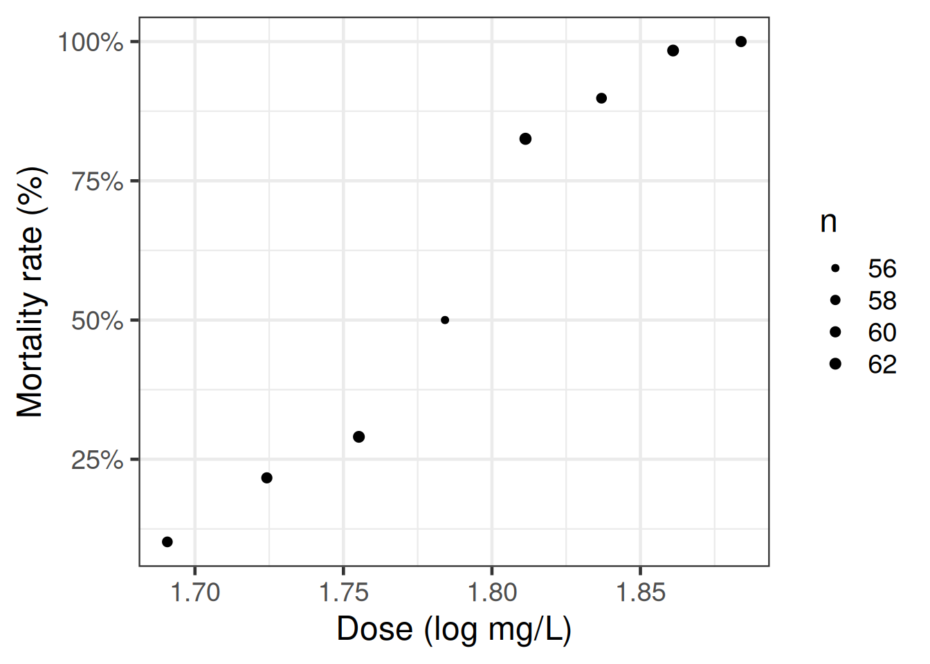
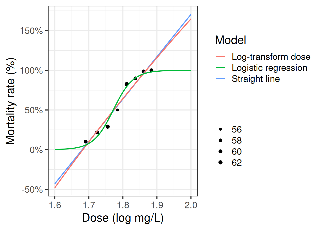
Consider the grouped-data logistic regression model for the beetles data (Table 2). At the middle (4th of 8) dose in the dataset, \(x = 1.7842\), the fitted log-odds of death is \(\hat{\eta} = 0.4277\), and the fitted probability of death is \(\hat{\pi} = \operatorname{expit}\mathopen{}\left\{0.4277\right\}\mathclose{} = 0.6053\). By Corollary 4, the slope of the expit function at this fitted log-odds value is:

\[ \operatorname{expit}'\mathopen{}\left\{0.4277\right\}\mathclose{} = 0.6053 \times (1 - 0.6053) = 0.2389 \]

That is, near dose \(x = 1.7842\), a small increase of \(\Delta\eta\) in the fitted log-odds corresponds to an increase of approximately \(0.2389 \times \Delta\eta\) in the fitted probability of death.

Summary matrix of derivatives

Each entry gives the derivative of the column quantity with respect to the row quantity; that is, the entry in row \(i\) and column \(j\) is \(\frac{\partial (\text{col } j)}{\partial (\text{row } i)}\).

Dimensions of each entry depend on the types of the row and column quantities:

• Scalar/scalar (upper-left \(3 \times 3\) block): row and column are both scalars (\(\pi\), \(\omega\), or \(\eta\)); derivative is a scalar.
• Gradient (lower-left \(2 \times 3\) block): row is a \(p\)-vector (\(\tilde{x}\) or \(\tilde{\beta}\)), column is a scalar; derivative is a \(p\)-vector (gradient).
• Jacobian (lower-right \(2 \times 2\) block): both row and column are \(p\)-vectors; derivative is a \(p \times p\) matrix.
• Undefined (upper-right \(3 \times 2\) block): row is a scalar (\(\pi\), \(\omega\), or \(\eta\)), column is \(\tilde{x}\) or \(\tilde{\beta}\). Each of these entries would be the derivative of a \(p\)-vector with respect to a scalar, which would require expressing \(\tilde{x}\) (or \(\tilde{\beta}\)) as a function of that scalar. No such function exists, because the map from the vector to the scalar is not invertible: for \(p > 1\), many distinct vectors produce the same value of \(\eta= \tilde{x} \cdot \tilde{\beta}\) (and hence the same \(\omega\) and \(\pi\)), so the scalar does not determine the vector, and these derivatives are undefined.

Table 6: Matrix of logistic regression derivatives (\(p\) = number of predictors, \(\eta\stackrel{\text{def}}{=}\tilde{x} \cdot \tilde{\beta}\), \(\omega\stackrel{\text{def}}{=}\operatorname{exp}\mathopen{}\left\{\eta\right\}\mathclose{}\), \(\pi\stackrel{\text{def}}{=}\omega/ (1 + \omega)\)). Each entry is the derivative of the column quantity with respect to the row quantity. Entries marked “undef” are not defined because the vector-to-scalar map is not invertible: the scalar row quantity does not determine the vector column quantity.

\[ \begin{array}{r|ccccc} & \pi& \omega& \eta& \tilde{x}& \tilde{\beta}\\ \hline \pi & 1 & \mathopen{}\left(1+\omega\right)^2\mathclose{} & \dfrac{\mathopen{}\left(1+\omega\right)^2\mathclose{}}{\omega} & \text{undef} & \text{undef} \\[10pt] \omega & \mathopen{}\left(1-\pi\right)^2\mathclose{} & 1 & \dfrac{1}{\omega} & \text{undef} & \text{undef} \\[10pt] \eta & \pi(1-\pi) & \omega & 1 & \text{undef} & \text{undef} \\[10pt] \tilde{x} & \underbrace{\tilde{\beta}\pi(1-\pi)}_{p \times 1} & \underbrace{\tilde{\beta}\omega}_{p \times 1} & \underbrace{\tilde{\beta}}_{p \times 1} & \underbrace{\mathbb{I}}_{p \times p} & \mathbf{0}_{p \times p} \\[10pt] \tilde{\beta} & \underbrace{\tilde{x}\pi(1-\pi)}_{p \times 1} & \underbrace{\tilde{x}\omega}_{p \times 1} & \underbrace{\tilde{x}}_{p \times 1} & \mathbf{0}_{p \times p} & \underbrace{\mathbb{I}}_{p \times p} \\ \end{array} \]

4 Understanding logistic regression models

Lemma 3 (Derivative of log-odds w.r.t. predictor) By the derivative of a linear combination:

\[ \begin{aligned} \frac{\partial \eta}{\partial \tilde{x}} &= \frac{\partial}{\partial \tilde{x}} \tilde{x}\cdot \tilde{\beta} \\ &= \tilde{\beta} \end{aligned} \]

Exercise 8 Consider a logistic regression model with a single predictor, \(X\):

\[ \begin{aligned} Y_i|X_i &\ \sim_{\perp\!\!\!\perp}\ \operatorname{Ber}(\pi(X_i)) \\ \pi(x) &= \operatorname{expit}\mathopen{}\left\{\eta(x)\right\}\mathclose{} = \pi(\omega(\eta(x))) \\ \eta(x) &= \alpha + \beta x \end{aligned} \tag{5}\]

Find the derivative of \(\pi(x) = \operatorname{E}\mathopen{}\left[Y|X=x\right]\mathclose{}\) with respect to \(x\):

\[\frac{\partial \pi}{\partial x} = ?\]

Solution 8. By Theorem 6, Lemma 3, and the chain rule:

\[ \begin{aligned} \frac{\partial \pi}{\partial x} &={\color{red}{\frac{\partial \pi}{\partial \eta}}} {\color{teal}{\frac{\partial \eta}{\partial x}}} \\ &= {\color{red}{\pi (1-\pi)}} {\color{teal}{\beta}} \\ &= {\color{red}{\operatorname{Var}\mathopen{}\left(Y|X=x\right)\mathclose{}}} \cdot {\color{teal}{\beta}} \end{aligned} \]

The slope is steepest at \(\pi = 0.5\), i.e., at \(\eta = 0\), which for a unipredictor model occurs at \(x = -\alpha/\beta\). The slope goes to 0 as \(x\) goes to \(-\infty\) or \(+\infty\) (compare with the graph of the expit function).

Note

See the general procedure for interpreting a regression coefficient for full details, including how to handle interaction terms and how to set remaining covariates to their reference values.

In order to interpret \(\beta_j\): differentiate or difference \({\color{red}{\eta(\tilde{x})}}\) with respect to \({\color{red}{x_j}}\) (depending on whether \(x_j\) is continuous or discrete, respectively):

\[\frac{\partial}{\partial {\color{red}{x_j}}} {\color{red}{\eta(\tilde{x})}}\]

In order to find the MLE \(\hat{\tilde{\beta}}\): differentiate the log-likelihood function \({\color{teal}{\ell(\tilde{\beta})}}\) with respect to \({\color{teal}{\tilde{\beta}}}\):

\[\frac{\partial}{\partial {\color{teal}{\tilde{\beta}}}} {\color{teal}{\ell(\tilde{\beta})}}\]

Exercise 9 (General formula for odds ratios in logistic regression) Consider the generic logistic regression model:

• \(Y_i|\tilde{X}_i \ \sim_{\perp\!\!\!\perp}\ \operatorname{Ber}(\pi(\tilde{X}_i))\)
• \(\operatorname{logit}\mathopen{}\left\{\pi(\tilde{x})\right\}\mathclose{} = \eta(\tilde{x})\)
• \(\eta(\tilde{x}) = \tilde{x}'\tilde{\beta}\)

Let \(\tilde{x}\) and \({\tilde{x}^*}\) be two covariate patterns, representing two individuals or two subpopulations.

Find a concise formula to compute the odds ratio comparing covariate patterns \(\tilde{x}\) and \({\tilde{x}^*}\):

\[\theta_{\omega}(\tilde{x},{\tilde{x}^*}) \stackrel{\text{def}}{=}\frac{\omega(\tilde{x})}{\omega({\tilde{x}^*})} \tag{6}\]

Solution 9 (General formula for odds ratios in logistic regression). \[ \begin{aligned} \theta_{\omega}(\tilde{x},{\tilde{x}^*}) &\stackrel{\text{def}}{=}\frac{\omega(\tilde{x})}{\omega({\tilde{x}^*})} \\ &= \frac{\operatorname{exp}\mathopen{}\left\{\eta(\tilde{x})\right\}\mathclose{}}{\operatorname{exp}\mathopen{}\left\{\eta({\tilde{x}^*})\right\}\mathclose{}} \\ &= \operatorname{exp}\mathopen{}\left\{{\color{red}{\eta(\tilde{x}) - \eta({\tilde{x}^*})}}\right\}\mathclose{} \end{aligned} \]

Solution 9 is more concrete than Equation 6, but it doesn’t yet completely explain how to compute \(\theta_{\omega}(\tilde{x},{\tilde{x}^*})\), so let’s mark it as a lemma:

Lemma 4 (General formula for odds ratios in logistic regression) \[\theta_{\omega}(\tilde{x},{\tilde{x}^*}) = \operatorname{exp}\mathopen{}\left\{{\color{red}{\eta(\tilde{x}) - \eta({\tilde{x}^*})}}\right\}\mathclose{} \tag{7}\]

Proof. By Solution 9.

Definition 2 (Difference in log-odds)  

Let \(\tilde{x}\) and \({\tilde{x}^*}\) be two covariate patterns, representing two individuals or two subpopulations.

Then we can define the difference in log-odds between \(\tilde{x}\) and \({\tilde{x}^*}\), denoted \(\Delta\eta(\tilde{x}, {\tilde{x}^*})\) or \(\Delta\eta\) for short, as:

\[{\color{red}{\Delta\eta}} \stackrel{\text{def}}{=}{\color{red}{\eta(\tilde{x}) - \eta({\tilde{x}^*})}}\]

Corollary 5 (Shorthand general formula for odds ratios in logistic regression) \[\theta_{\omega}(\tilde{x},{\tilde{x}^*}) = \operatorname{exp}\mathopen{}\left\{{\color{red}{\Delta\eta}}\right\}\mathclose{} \tag{8}\]

Proof. By Lemma 4 and Definition 2.

Exercise 10 (Difference in log-odds) Find a concise expression for the difference in log-odds: \[\Delta\eta\stackrel{\text{def}}{=}{\color{red}{\eta(\tilde{x}) - \eta({\tilde{x}^*})}}\]

Solution 10 (Difference in log-odds). \[ \begin{aligned} {\color{red}{\Delta\eta}} &\stackrel{\text{def}}{=}{\color{red}{\eta(\tilde{x}) - \eta({\tilde{x}^*})}} \\ &= (\tilde{x}\cdot\tilde{\beta}) - ({\tilde{x}^*}\cdot\tilde{\beta}) \\ &= (\tilde{x}^{\top}\tilde{\beta}) - (\mathopen{}\left({\tilde{x}^*}\right)\mathclose{}^{\top}\tilde{\beta}) \\ &= (\tilde{x}^{\top} - \mathopen{}\left({\tilde{x}^*}\right)\mathclose{}^{\top})\tilde{\beta} \\ &= (\tilde{x}- {\tilde{x}^*})^{\top}\tilde{\beta} \\ &= ({\color{teal}{\tilde{x}- {\tilde{x}^*}}})\cdot\tilde{\beta} \end{aligned} \]

Lemma 5 (Difference in log-odds) \[{\color{red}{\Delta\eta}}= ({\color{teal}{\tilde{x}- {\tilde{x}^*}}})\cdot\tilde{\beta}\]

Proof. By Solution 10.

Definition 3 (Difference in covariate patterns)  

Let \(\tilde{x}\) and \({\tilde{x}^*}\) be two covariate patterns, representing two individuals or two subpopulations. The difference in covariate patterns, denoted \(\Delta\tilde{x}\), is defined as:

\[{\color{teal}{\Delta\tilde{x}}} \stackrel{\text{def}}{=}{\color{teal}{\tilde{x}- {\tilde{x}^*}}}\]

Corollary 6 (Difference in log-odds) \[{\color{red}{\Delta\eta}}= ({\color{teal}{\Delta\tilde{x}}}) \cdot \tilde{\beta}\]

Proof. By Lemma 5 and Definition 3.

Exercise 11 Find an expression for the odds ratio \(\theta_{\omega}(\tilde{x},{\tilde{x}^*})\) in terms of \(\Delta\tilde{x}\) and \(\tilde{\beta}\).

Solution 11. Combine Corollary 5 and Corollary 6:

\[ \begin{aligned} \theta_{\omega}(\tilde{x},{\tilde{x}^*}) &= \operatorname{exp}\mathopen{}\left\{\Delta\eta\right\}\mathclose{} \\ &= \operatorname{exp}\mathopen{}\left\{\Delta\tilde{x}\cdot \tilde{\beta}\right\}\mathclose{} \end{aligned} \]

Theorem 7 (Odds ratio from difference in covariate patterns) The odds ratio comparing covariate patterns \(\tilde{x}\) and \({\tilde{x}^*}\) is:

\[\theta_{\omega}(\tilde{x},{\tilde{x}^*}) = \operatorname{exp}\mathopen{}\left\{(\Delta\tilde{x}) \cdot \tilde{\beta}\right\}\mathclose{} \tag{9}\]

Proof. By Solution 11.

Example 2 (Odds ratio between adjacent beetle dose levels)  

We can apply Theorem 7 to the beetles logistic regression model (Table 2).

The estimated dose coefficient for that model is \(\hat{\beta}_1 = 34.270326\).

Consider the two covariate patterns given by the two lowest dose levels in the beetles data: \(\tilde{x}= (1, 1.7242)^{\top}\) and \({\tilde{x}^*}= (1, 1.6907)^{\top}\) (intercept and dose). Their difference is \(\Delta\tilde{x}= \tilde{x}- {\tilde{x}^*}= (0, 0.0335)^{\top}\).

By Theorem 7, the estimated odds ratio comparing these two dose levels is:

\[ \begin{aligned} \hat{\theta_{\omega}}(\tilde{x},{\tilde{x}^*}) &= \operatorname{exp}\mathopen{}\left\{(\Delta\tilde{x})\cdot \hat{\beta}\right\}\mathclose{} && \text{(@thm-logistic-OR)} \\ &= \operatorname{exp}\mathopen{}\left\{0\cdot\hat{\beta}_0 + (0.0335)\cdot \hat{\beta}_1\right\}\mathclose{} && \text{(expand the dot product)} \\ &= \operatorname{exp}\mathopen{}\left\{(0.0335)\cdot (34.270326)\right\}\mathclose{} && \text{(substitute } \hat{\beta}_1\text{)} \\ &= 3.152059 && \text{(evaluate the exponential)} \end{aligned} \]

So an increase of \(0.0335\) units in dose (the gap between the two lowest dose levels) multiplies the estimated odds of death by about \(3.15\).

Corollary 7 (Log odds ratio equals the difference in log-odds) \[\operatorname{log}\mathopen{}\left\{\theta_{\omega}(\tilde{x},{\tilde{x}^*})\right\}\mathclose{} = \Delta\eta\]

5 Estimating logistic regression models

Model

Assume:

• \(Y_i|\tilde{X}_i \ \sim_{\perp\!\!\!\perp}\ \operatorname{Ber}(\pi(X_i))\)
• \(\pi(\tilde{x}) = \operatorname{expit}\mathopen{}\left\{\eta(\tilde{x})\right\}\mathclose{}\)
• \(\eta(\tilde{x}) = \tilde{x}\cdot \tilde{\beta}\)

Likelihood function

Exercise 12 Compute and graph the likelihood for the beetles data model:

library(glmx)
library(dplyr)
data(BeetleMortality)
beetles <- BeetleMortality |>
  mutate(
    pct = died / n,
    survived = n - died,
    dose_c = dose - mean(dose)
  )
beetles_long <-
  beetles |>
  reframe(
    .by = everything(),
    outcome = c(
      rep(1, times = died),
      rep(0, times = survived)
    )
  )
beetles

Table 7: Mortality rates of adult flour beetles after five hours’ exposure to gaseous carbon disulphide (Bliss 1935)

beetles_glm <-
  beetles |>
  glm(
    formula = cbind(died, survived) ~ dose,
    family = "binomial"
  )
equatiomatic::extract_eq(beetles_glm)

\[ \log\left[ \frac { P( \operatorname{died} = \operatorname{60} ) }{ 1 - P( \operatorname{died} = \operatorname{60} ) } \right] = \alpha + \beta_{1}(\operatorname{dose}) \]

beetles_glm |>
  parameters::parameters() |>
  parameters::print_md()

Table 8: Fitted logistic regression model for beetles data

Parameter	Log-Odds	SE	95% CI	z	p
(Intercept)	-60.72	5.18	(-71.44, -51.08)	-11.72	< .001
dose	34.27	2.91	(28.85, 40.30)	11.77	< .001

Solution 12.

odds_inv <- function(omega) (1 + omega^-1)^-1
lik_beetles0 <- function(beta_0, beta_1) {
  beetles |>
    mutate(
      eta = beta_0 + beta_1 * dose,
      omega = exp(eta),
      pi = odds_inv(omega),
      Lik = pi^died * (1 - pi)^survived,
      # llik = died*eta + n*log(1 - pi)
    ) |>
    pull(Lik) |>
    prod()
}

lik_beetles <- Vectorize(lik_beetles0)

ranges <- beetles_glm |> confint.default(level = 0.05)

n_points <- 25
beta_0s <- seq(
  ranges["(Intercept)", 1],
  ranges["(Intercept)", 2],
  length.out = n_points
)
beta_1s <- seq(
  ranges["dose", 1],
  ranges["dose", 2],
  length.out = n_points
)
names(beta_0s) <- round(beta_0s, 2)
names(beta_1s) <- round(beta_1s, 2)

if (run_graphs) {
  lik_mat_beetles <- outer(beta_0s, beta_1s, lik_beetles)
  plotly::plot_ly(
    type = "surface",
    x = ~beta_0s,
    y = ~beta_1s,
    z = ~ t(lik_mat_beetles)
  )
  # see https://stackoverflow.com/questions/69472185/correct-use-of-coordinates-to-plot-surface-data-with-plotly 
  # for explanation of why transpose `t()` is needed
  
}

Figure 6: Likelihood of beetles data. Bumps on ridge are artifacts of render; increase n_points to improve render quality.

Log-likelihood function

Exercise 13 Find the log-likelihood function for the general logistic regression model.

Solution 13. \[ \begin{aligned} \ell(\tilde{\beta}, \tilde{y}) &\stackrel{\text{def}}{=}\operatorname{log}\mathopen{}\left\{\mathcal{L}(\tilde{\beta}, \tilde{y}) \right\}\mathclose{} && \text{(definition of log-likelihood)} \\ &= \operatorname{log}\mathopen{}\left\{\prod_{i=1}^n\mathcal{L}_i(\tilde{\beta}, y_i)\right\}\mathclose{} && \text{(likelihood factors, by independence)} \\ &= \sum_{i=1}^n\operatorname{log}\mathopen{}\left\{\mathcal{L}_i(\tilde{\beta}, y_i)\right\}\mathclose{} && \text{(log of a product is the sum of the logs)} \\ &= \sum_{i=1}^n{\color{red}{\ell_i}}(\pi(\tilde{x}_i)) && \text{(definition: } {\color{red}{\ell_i}} \stackrel{\text{def}}{=}\operatorname{log}\mathopen{}\left\{\mathcal{L}_i\right\}\mathclose{} \text{)} \end{aligned} \tag{10}\]

Using log-odds as a function of probability and one plus odds in terms of non-event probability:

\[ \begin{aligned} {\color{red}{\ell_i}}(\pi_i) &= y_i \operatorname{log}\mathopen{}\left\{\pi_i\right\}\mathclose{} + (1 - y_i) \operatorname{log}\mathopen{}\left\{1-\pi_i\right\}\mathclose{} && \text{(log of the Bernoulli likelihood } \pi_i^{y_i}(1-\pi_i)^{1-y_i} \text{)} \\ &= y_i \operatorname{log}\mathopen{}\left\{\pi_i\right\}\mathclose{} + 1 \cdot\operatorname{log}\mathopen{}\left\{1-\pi_i\right\}\mathclose{} - y_i \cdot\operatorname{log}\mathopen{}\left\{1-\pi_i\right\}\mathclose{} && \text{(distribute } (1-y_i) \text{)} \\ &= y_i \operatorname{log}\mathopen{}\left\{\pi_i\right\}\mathclose{} + \operatorname{log}\mathopen{}\left\{1-\pi_i\right\}\mathclose{} - y_i \operatorname{log}\mathopen{}\left\{1-\pi_i\right\}\mathclose{} && \text{(multiplicative identity: } 1 \cdot\operatorname{log}\mathopen{}\left\{1-\pi_i\right\}\mathclose{} = \operatorname{log}\mathopen{}\left\{1-\pi_i\right\}\mathclose{} \text{)} \\ &= y_i \operatorname{log}\mathopen{}\left\{\pi_i\right\}\mathclose{} - y_i \operatorname{log}\mathopen{}\left\{{\color{teal}{1-\pi_i}}\right\}\mathclose{} + \operatorname{log}\mathopen{}\left\{1-\pi_i\right\}\mathclose{} && \text{(commute the addition)} \\ &= y_i \mathopen{}\left(\operatorname{log}\mathopen{}\left\{{\color{red}{\pi_i}}\right\}\mathclose{} - \operatorname{log}\mathopen{}\left\{{\color{teal}{1-\pi_i}}\right\}\mathclose{}\right)\mathclose{} + \operatorname{log}\mathopen{}\left\{1-\pi_i\right\}\mathclose{} && \text{(factor out } y_i \text{)} \\ &= y_i \operatorname{log}\mathopen{}\left\{\frac{{\color{red}{\pi_i}}}{{\color{teal}{1-\pi_i}}}\right\}\mathclose{} + \operatorname{log}\mathopen{}\left\{1-\pi_i\right\}\mathclose{} && \text{(difference of logs is the log of the quotient)} \\ &= y_i \operatorname{logit}(\pi_i) + \operatorname{log}\mathopen{}\left\{1-\pi_i\right\}\mathclose{} && \text{(log-odds identity: } \operatorname{logit}(\pi) = \operatorname{log}\mathopen{}\left\{\pi/(1-\pi)\right\}\mathclose{} \text{)} \\ &= y_i \eta_i + \operatorname{log}\mathopen{}\left\{1-\pi_i\right\}\mathclose{} && \text{(definition: } \eta_i \stackrel{\text{def}}{=}\operatorname{logit}(\pi_i) \text{)} \\ &= y_i \eta_i + \operatorname{log}\mathopen{}\left\{\mathopen{}\left(1+\omega_i\right)^{-1}\mathclose{}\right\}\mathclose{} && \text{(non-event probability: } 1-\pi_i = \mathopen{}\left(1+\omega_i\right)^{-1}\mathclose{} \text{)} \\ &= y_i \eta_i - \operatorname{log}\mathopen{}\left\{1+\omega_i\right\}\mathclose{} && \text{(log of a reciprocal)} \end{aligned} \]

Lemma 6 (Per-observation log-likelihood component) \[\ell_i(\pi_i) = y_i \eta_i - \operatorname{log}\mathopen{}\left\{1+\omega_i\right\}\mathclose{}\]

Exercise 14 Compute and graph the log-likelihood for the beetles data.

Solution 14.

odds_inv <- function(omega) (1 + omega^-1)^-1
llik_beetles0 <- function(beta_0, beta_1) {
  beetles |>
    mutate(
      eta = beta_0 + beta_1 * dose,
      omega = exp(eta),
      pi = odds_inv(omega), # need for next line:
      llik = died*eta + n*log(1 - pi)
    ) |>
    pull(llik) |>
    sum()
}

llik_beetles <- Vectorize(llik_beetles0)

# to check that we implemented it correctly:
# ests = coef(beetles_glm_ungrouped)
# logLik(beetles_glm_ungrouped)
# llik_beetles(ests[1], ests[2])

if (run_graphs) {
  llik_mat_beetles <- outer(beta_0s, beta_1s, llik_beetles)
  plotly::plot_ly(
    type = "surface",
    x = ~beta_0s,
    y = ~beta_1s,
    z = ~ t(llik_mat_beetles)
  )
}

Figure 7: log-likelihood of beetles data

Let’s center dose:

beetles_glm_grouped_centered <- beetles |>
  glm(
    formula = cbind(died, survived) ~ dose_c,
    family = "binomial"
  )

beetles_glm_ungrouped_centered <- beetles_long |>
  mutate(died = outcome) |>
  glm(
    formula = died ~ dose_c,
    family = "binomial"
  )

equatiomatic::extract_eq(beetles_glm_ungrouped_centered)

\[ \log\left[ \frac { P( \operatorname{died} = \operatorname{1} ) }{ 1 - P( \operatorname{died} = \operatorname{1} ) } \right] = \alpha + \beta_{1}(\operatorname{dose\_c}) \]

beetles_glm_grouped_centered |>
  parameters::parameters() |>
  parameters::print_md()

Table 9: Fitted logistic regression model for beetles data, with dose centered

Parameter	Log-Odds	SE	95% CI	z	p
(Intercept)	0.74	0.14	(0.48, 1.02)	5.40	< .001
dose c	34.27	2.91	(28.85, 40.30)	11.77	< .001

odds_inv <- function(omega) (1 + omega^-1)^-1
lik_beetles0 <- function(beta_0, beta_1) {
  beetles |>
    mutate(
      eta = beta_0 + beta_1 * dose_c,
      omega = exp(eta),
      pi = odds_inv(omega),
      Lik = (pi^died) * (1 - pi)^(survived)
    ) |>
    pull(Lik) |>
    prod()
}

lik_beetles <- Vectorize(lik_beetles0)

ranges <- beetles_glm_grouped_centered |> confint.default(level = .95)

n_points <- 25
beta_0s <- seq(
  ranges["(Intercept)", 1],
  ranges["(Intercept)", 2],
  length.out = n_points
)
beta_1s <- seq(
  ranges["dose_c", 1],
  ranges["dose_c", 2],
  length.out = n_points
)
names(beta_0s) <- round(beta_0s, 2)
names(beta_1s) <- round(beta_1s, 2)
if (run_graphs) {
  lik_mat_beetles <- outer(beta_0s, beta_1s, lik_beetles)
  plotly::plot_ly(
    type = "surface",
    x = ~beta_0s,
    y = ~beta_1s,
    z = ~ t(lik_mat_beetles)
  )
}

Figure 8: Likelihood of beetles data (centered model)

odds_inv <- function(omega) (1 + omega^-1)^-1
llik_beetles0 <- function(beta_0, beta_1) {
  beetles |>
    mutate(
      eta = beta_0 + beta_1 * dose_c,
      omega = exp(eta),
      pi = odds_inv(omega),
      llik = died * eta + n*log(1 - pi)
    ) |>
    pull(llik) |>
    sum()
}

llik_beetles <- Vectorize(llik_beetles0)

if (run_graphs) {
  llik_mat_beetles <- outer(beta_0s, beta_1s, llik_beetles)
  plotly::plot_ly(
    type = "surface",
    x = ~beta_0s,
    y = ~beta_1s,
    z = ~ t(llik_mat_beetles)
  )
}

Figure 9: log-likelihood of beetles data (centered model)

Score function

As usual, by independence, we have:

Lemma 7 (Score function decomposes over observations) \[ \begin{aligned} {\color{brown}{\tilde{\ell'}(\tilde{\beta})}} &\stackrel{\text{def}}{=}\frac{\partial}{\partial \tilde{\beta}} \ell(\tilde{\beta}) && \text{(definition of the score function)} \\ &= \frac{\partial}{\partial \tilde{\beta}} \sum_{i=1}^n\ell_i(\tilde{\beta}) && \text{(the log-likelihood decomposes over observations, by independence)} \\ &= \sum_{i=1}^n\frac{\partial}{\partial \tilde{\beta}} \ell_i(\tilde{\beta}) && \text{(linearity of differentiation)} \\ &= \sum_{i=1}^n{\color{magenta}{\tilde{\ell'_i}(\tilde{\beta})}} && \text{(definition: } {\color{magenta}{\tilde{\ell'_i}}} \stackrel{\text{def}}{=}\frac{\partial}{\partial \tilde{\beta}} \ell_i \text{)} \end{aligned} \]

Starting from Lemma 6, we can apply the vector chain rule:

Lemma 8 (Chain rule applied to the score component) \[ \begin{aligned} {\color{magenta}{\tilde{\ell_i'}(\tilde{\beta})}} &\stackrel{\text{def}}{=}\frac{\partial}{\partial \tilde{\beta}} \ell_i(\tilde{\beta}) && \text{(definition of the score component)} \\ &= \frac{\partial}{\partial \tilde{\beta}}\mathopen{}\left(y_i \eta_i - \operatorname{log}\mathopen{}\left\{1+\omega_i\right\}\mathclose{}\right)\mathclose{} && \text{(per-observation log-likelihood)} \\ &= \frac{\partial}{\partial \tilde{\beta}}\mathopen{}\left(y_i\eta_i\right)\mathclose{} - \frac{\partial}{\partial \tilde{\beta}}\operatorname{log}\mathopen{}\left\{1+\omega_i\right\}\mathclose{} && \text{(linearity of differentiation)} \\ &= {\color{red}{\frac{\partial \eta_i}{\partial \tilde{\beta}}}}y_i - \frac{\partial}{\partial \tilde{\beta}}\operatorname{log}\mathopen{}\left\{1+\omega_i\right\}\mathclose{} && \text{(constant-factor rule: } y_i \text{ does not depend on } \tilde{\beta}\text{)} \\ &= {\color{red}{\frac{\partial \eta_i}{\partial \tilde{\beta}}}}y_i - \frac{\partial u_i}{\partial \tilde{\beta}} \mathopen{}\left(\frac{\partial}{\partial u_i}\operatorname{log}\mathopen{}\left\{u_i\right\}\mathclose{}\right)\mathclose{} && \text{(vector chain rule, with } u_i \stackrel{\text{def}}{=}1+\omega_i \text{)} \\ &= {\color{red}{\frac{\partial \eta_i}{\partial \tilde{\beta}}}}y_i - \frac{\partial u_i}{\partial \tilde{\beta}} \frac{1}{u_i} && \text{(derivative of the natural log: } \frac{\partial}{\partial u}\operatorname{log}\mathopen{}\left\{u\right\}\mathclose{} = 1/u \text{)} \\ &= {\color{red}{\frac{\partial \eta_i}{\partial \tilde{\beta}}}}y_i - {\color{purple}{\frac{\partial \omega_i}{\partial \tilde{\beta}}}} \frac{1}{u_i} && \text{(} \frac{\partial u_i}{\partial \tilde{\beta}} = \frac{\partial \omega_i}{\partial \tilde{\beta}} \text{: the constant 1 has derivative } \mathbf{0}_{(p+1) \times 1} \text{)} \\ &= {\color{red}{\frac{\partial \eta_i}{\partial \tilde{\beta}}}}y_i - {\color{purple}{\frac{\partial \omega_i}{\partial \tilde{\beta}}}}\frac{1}{1+\omega_i} && \text{(substitute back } u_i = 1+\omega_i \text{)} \end{aligned} \]

Lemma 9 (Derivative of log-odds with respect to coefficients) By the derivative of a linear combination:

\[ \begin{aligned} {\color{red}{\frac{\partial \eta}{\partial \tilde{\beta}}}} &= \frac{\partial}{\partial \tilde{\beta}}(\tilde{x}\cdot \tilde{\beta}) \\ &= {\color{red}{\tilde{x}}} \end{aligned} \tag{11}\]

Lemma 9 is very similar to Lemma 3, but not quite the same; Lemma 3 differentiates by \(\tilde{x}\), whereas Lemma 9 differentiates by \(\tilde{\beta}\).

Theorem 8 (Gradient of odds w.r.t. coefficients)  

To derive \(\frac{\partial \omega}{\partial \tilde{\beta}}\), we can apply the vector chain rule again along with Lemma 2 and Lemma 9:

\[ \begin{aligned} \frac{\partial \omega}{\partial \tilde{\beta}} &= {\color{red}{\frac{\partial \eta}{\partial \tilde{\beta}}}} {\color{teal}{\frac{\partial \omega}{\partial \eta}}} && \text{(vector chain rule, through } \eta= \eta \text{)} \\ &= {\color{red}{\tilde{x}}} {\color{teal}{\frac{\partial \omega}{\partial \eta}}} && \text{(gradient of log-odds w.r.t. coefficients: } \frac{\partial \eta}{\partial \tilde{\beta}} = \tilde{x}\text{)} \\ &= {\color{red}{\tilde{x}}} {\color{teal}{\omega}} && \text{(derivative of odds w.r.t. log-odds: } \frac{\partial \omega}{\partial \eta} = \omega\text{)} \end{aligned} \]

Corollary 8 (Gradient of odds w.r.t. coefficients in terms of probability) \[ \begin{aligned} \frac{\partial \omega}{\partial \tilde{\beta}} &= {\color{red}{\tilde{x}}} {\color{teal}{\omega}} && \text{(gradient of odds w.r.t. coefficients)} \\ &= {\color{red}{\tilde{x}}} \frac{\pi}{1-\pi} && \text{(odds in terms of probability: } \omega= \frac{\pi}{1-\pi} \text{)} \end{aligned} \]

Now we can combine Lemma 8, Lemma 9, and Theorem 8:

\[ \begin{aligned} {\color{magenta}{\ell_i'(\tilde{\beta})}} &= {\color{red}{\frac{\partial \eta_i}{\partial \tilde{\beta}}}}y_i - {\color{purple}{\frac{\partial \omega_i}{\partial \tilde{\beta}}}}\frac{1}{1+\omega_i} && \text{(score component lemma)} \\ &= {\color{red}{\tilde{x}_i}}y_i - {\color{purple}{\frac{\partial \omega_i}{\partial \tilde{\beta}}}}\frac{1}{1+\omega_i} && \text{(gradient of log-odds w.r.t. coefficients: } \frac{\partial \eta_i}{\partial \tilde{\beta}} = \tilde{x}_i \text{)} \\ &= {\color{red}{\tilde{x}_i}}y_i - {\color{red}{\tilde{x}_i}} {\color{teal}{\omega_i}}\frac{1}{1+\omega_i} && \text{(gradient of odds w.r.t. coefficients: } \frac{\partial \omega_i}{\partial \tilde{\beta}} = \tilde{x}_i \omega_i \text{)} \\ &= {\color{red}{\tilde{x}_i}}y_i - {\color{red}{\tilde{x}_i}} \frac{{\color{teal}{\omega_i}}}{1+\omega_i} && \text{(combine the scalar factors into one fraction)} \\ &= \tilde{x}_i y_i - \tilde{x}_i \pi_i && \text{(inverse-odds identity: } \frac{\omega_i}{1+\omega_i} = \pi_i \text{)} \\ &= \tilde{x}_i (y_i - \pi_i) && \text{(factor out } \tilde{x}_i \text{)} \\ &= \tilde{x}_i (y_i - \mu_i) && \text{(Bernoulli conditional mean: } \pi_i = \mu_i \text{)} \\ &= \tilde{x}_i (y_i - \operatorname{E}[Y_i|\tilde{X}_i=\tilde{x}_i]) && \text{(definition: } \mu_i \stackrel{\text{def}}{=}\operatorname{E}[Y_i|\tilde{X}_i=\tilde{x}_i] \text{)} \\ &= \tilde{x}_i \ \varepsilon(y_i|\tilde{X}_i=\tilde{x}_i) && \text{(definition of the error: } \varepsilon(y|\tilde{X}=\tilde{x}) \stackrel{\text{def}}{=}y - \operatorname{E}[Y|\tilde{X}=\tilde{x}] \text{)} \\ &= {\color{magenta}{\tilde{x}_i \varepsilon_i}} && \text{(abbreviation: } \varepsilon_i \stackrel{\text{def}}{=}\varepsilon(y_i|\tilde{X}_i=\tilde{x}_i) \text{)} \end{aligned} \]

Theorem 9 (Score component for one observation) \[{\color{magenta}{\ell_i'(\tilde{\beta})}} = {\color{magenta}{\tilde{x}_i \varepsilon_i}} \tag{12}\]

This last expression is essentially the same as we found in linear regression.

Finally, combining Lemma 7 and Theorem 9, we have:

Theorem 10 (Logistic-model score function) \[ \begin{aligned} {\color{brown}{\tilde{\ell'}(\tilde{\beta})}} &= \sum_{i=1}^n{\color{magenta}{\ell_i'(\tilde{\beta})}} && \text{(the score decomposes over observations)} \\ &= \sum_{i=1}^n\underbrace{\tilde{x}_i}_{(p+1) \times 1} \underbrace{\varepsilon_i}_{1 \times 1} && \text{(score component for one observation)} \\ &= {\color{brown}{\underbrace{\mathbf{X}^{\top}}_{(p+1) \times n} \underbrace{\tilde{\varepsilon}}_{n \times 1}}} && \text{(matrix form: } \sum_{i=1}^n\tilde{x}_i \varepsilon_i = \mathbf{X}^{\top}\tilde{\varepsilon}\text{)} \end{aligned} \tag{13}\]

The score function is vector-valued; its components are:

\[ \frac{\partial \ell}{\partial \tilde{\beta}} = \begin{pmatrix} \frac{\partial \ell}{\partial \beta_0} \\ \frac{\partial \ell}{\partial \beta_1} \\ \vdots \\ \frac{\partial \ell}{\partial \beta_p} \end{pmatrix} = \begin{pmatrix} \sum_{i=1}^n1 \varepsilon_i \\ \sum_{i=1}^nx_{i,1}\varepsilon_i \\ \vdots \\ \sum_{i=1}^nx_{i,p} \varepsilon_i \end{pmatrix} = \begin{pmatrix} \tilde{1} \cdot \tilde{\varepsilon} \\ \mathbf{X}_{\cdot 1} \cdot \tilde{\varepsilon} \\ \vdots \\ \mathbf{X}_{\cdot p} \cdot \tilde{\varepsilon}\end{pmatrix} \]

Here, \(\mathbf{X}_{\cdot j} \stackrel{\text{def}}{=}(x_{1j}, \ldots, x_{nj})\) denotes the \(j^{th}\) column of the design matrix \(\mathbf{X}\) (the \(n\)-vector of covariate \(j\)’s values across all observations), in contrast with \(\tilde{x}_i\), which denotes observation \(i\)’s covariate row vector (a \(p\)-vector).

Thus, the score equation \(\tilde{\ell'} = \mathbf{0}_{(p+1) \times 1}\) means that for the MLE \(\hat{\tilde{\beta}}\):

1. the sum of the errors (aka deviations) equals 0:

\[\sum_{i=1}^n\varepsilon_i = 0\]

2. the sums of the errors times each covariate also equal 0:

\[\mathbf{X}_{\cdot j} \cdot \tilde{\varepsilon}= \sum_{i=1}^nx_{ij} \varepsilon_i = 0, \forall j \in \mathopen{}\left\{1:p\right\}\mathclose{}\]

Example 3 In our model for the beetles data, we only have an intercept plus one covariate, gas concentration (\(c\)): \[\tilde{x}= (1, c)\]

If \(c_i\) is the gas concentration for the beetle in observation \(i\), and \(\tilde{c} = (c_1, c_2, ...c_n)\), then the score equation \(\tilde{\ell'} = \mathbf{0}_{2 \times 1}\) means that for the MLE \(\hat{\tilde{\beta}}\):

1. the sum of the errors (aka deviations) equals 0:

\[\sum_{i=1}^n\varepsilon_i = 0\]

2. the weighted sum of the error times the gas concentrations equals 0:

\[\sum_{i=1}^nc_i \varepsilon_i = 0 \]

Exercise 15 Implement and graph the score function for the beetles data

Solution 15.

odds_inv <- function(omega) (1 + omega^-1)^-1

score_fn_beetles_beta0_0 <- function(beta_0, beta_1) {
  beetles |>
    mutate(
      eta = beta_0 + beta_1 * dose_c,
      omega = exp(eta),
      pi = odds_inv(omega),
      mu = pi * n,
      epsilon = died - mu,
      score = epsilon
    ) |>
    pull(score) |>
    sum()
}
score_fn_beetles_beta_0 <- Vectorize(score_fn_beetles_beta0_0)

score_fn_beetles_beta1_0 <- function(beta_0, beta_1) {
  beetles |>
    mutate(
      eta = beta_0 + beta_1 * dose_c,
      omega = exp(eta),
      pi = odds_inv(omega),
      mu = pi * n,
      epsilon = died - mu,
      score = dose_c * epsilon
    ) |>
    pull(score) |>
    sum()
}
score_fn_beetles_beta_1 <- Vectorize(score_fn_beetles_beta1_0)

if (run_graphs) {
  scores_beetles_beta_0 <- outer(beta_0s, beta_1s, score_fn_beetles_beta_0)
  scores_beetles_beta_1 <- outer(beta_0s, beta_1s, score_fn_beetles_beta_1)

  plotly::plot_ly(
    x = ~beta_0s,
    y = ~beta_1s
  ) |>
    plotly::add_markers(
      type = "scatter",
      x = coef(beetles_glm_grouped_centered)["(Intercept)"],
      y = coef(beetles_glm_grouped_centered)["dose_c"],
      z = 0,
      marker = list(color = "black"),
      name = "MLE"
    ) |>
    plotly::add_surface(
      z = ~ t(scores_beetles_beta_1),
      name = "score_beta_1",
      colorscale = list(c(0, 1), c("red", "green")),
      showscale = FALSE,
      contours = list(
        z = list(
          show = TRUE,
          start = -1,
          end = 1,
          size = .1
        )
      ),
      opacity = 0.75
    ) |>
    plotly::add_surface(
      z = ~ t(scores_beetles_beta_0),
      colorscale = list(c(0, 1), c("yellow", "blue")),
      showscale = FALSE,
      contours = list(
        z = list(
          show = TRUE,
          start = -14,
          end = 14,
          size = 2
        )
      ),
      opacity = 0.75,
      name = "score_beta_0"
    ) |>
    plotly::layout(legend = list(orientation = "h"))
}

Figure 10: score functions of beetles data (centered model), by parameter (\(\beta_0\) and \(\beta_1\)), with MLE marked in black.

Hessian function

\[ \underbrace{\ell''(\tilde{\beta})}_{(p+1) \times (p+1)} = \sum_{i=1}^n\underbrace{{\color{olive}{\ell''_i(\tilde{\beta})}}}_{(p+1) \times (p+1)} \tag{14}\]

\[ \begin{aligned} {\color{olive}{\ell''_i(\tilde{\beta})}} &\stackrel{\text{def}}{=}\frac{\partial}{\partial \tilde{\beta}^{\top}}\tilde{\ell_i'} && \text{(definition of the Hessian component)} \\ &= \frac{\partial}{\partial \tilde{\beta}^{\top}}\mathopen{}\left(\tilde{x}_i\varepsilon_i\right)\mathclose{} && \text{(score component for one observation)} \\ &= \tilde{x}_i \frac{\partial}{\partial \tilde{\beta}^{\top}}\varepsilon_i && \text{(constant-factor rule: } \tilde{x}_i \text{ does not depend on } \tilde{\beta}\text{)} \\ &= \tilde{x}_i {\color{violet}{\varepsilon_i'}} && \text{(definition: } {\color{violet}{\varepsilon_i'}} \stackrel{\text{def}}{=}\frac{\partial}{\partial \tilde{\beta}^{\top}}\varepsilon_i \text{)} \end{aligned} \tag{15}\]

Theorem 11 (Gradient of fitted probability w.r.t. coefficients) Using Lemma 9 and Theorem 6:

\[ \begin{aligned} \frac{\partial \pi}{\partial \tilde{\beta}} &= {\color{red}{\frac{\partial \eta}{\partial \tilde{\beta}}}} {\color{teal}{\frac{\partial \pi}{\partial \eta}}} && \text{(vector chain rule, through } \eta\text{)} \\ &= {\color{red}{\tilde{x}}} {\color{teal}{\frac{\partial \pi}{\partial \eta}}} && \text{(gradient of log-odds w.r.t. coefficients: } \frac{\partial \eta}{\partial \tilde{\beta}} = \tilde{x}\text{)} \\ &= {\color{red}{\tilde{x}}} {\color{teal}{\pi(1-\pi)}} && \text{(derivative of probability w.r.t. log-odds: } \frac{\partial \pi}{\partial \eta} = \pi(1-\pi) \text{)} \end{aligned} \]

Using Theorem 11:

\[ \begin{aligned} {\color{violet}{\varepsilon'_i}} &\stackrel{\text{def}}{=}\frac{\partial \varepsilon_i}{\partial \tilde{\beta}^{\top}} && \text{(definition of } {\color{violet}{\varepsilon'_i}} \text{)} \\ &= \frac{\partial}{\partial \tilde{\beta}^{\top}}(y_i - \mu_i) && \text{(definition of the error: } \varepsilon_i \stackrel{\text{def}}{=}y_i - \mu_i \text{)} \\ &= \frac{\partial}{\partial \tilde{\beta}^{\top}}y_i - \frac{\partial}{\partial \tilde{\beta}^{\top}}\mu_i && \text{(linearity of differentiation)} \\ &= \mathbf{0}_{1 \times (p+1)} - \frac{\partial}{\partial \tilde{\beta}^{\top}}\mu_i && \text{(} y_i \text{ does not depend on } \tilde{\beta}\text{)} \\ &= -\frac{\partial \mu_i}{\partial \tilde{\beta}^{\top}} && \text{(additive identity)} \\ &= -{\color{purple}{\frac{\partial \pi_i}{\partial \tilde{\beta}^{\top}}}} && \text{(Bernoulli conditional mean: } \mu_i = \pi_i \text{)} \\ &= - \pi_i (1-\pi_i) \tilde{x}_i^{\top} && \text{(transpose of the gradient of } \pi \text{ w.r.t. coefficients)} \\ &= - \operatorname{Var}\mathopen{}\left(Y_i|\tilde{X}_i=\tilde{x}_i\right)\mathclose{} \tilde{x}_i^{\top} && \text{(Bernoulli conditional variance: } \operatorname{Var}\mathopen{}\left(Y_i|\tilde{X}_i=\tilde{x}_i\right)\mathclose{} = \pi_i(1-\pi_i) \text{)} \end{aligned} \]

Returning to Equation 15:

\[ \begin{aligned} {\color{olive}{\ell''_i(\tilde{\beta})}} &= \tilde{x}_i {\color{violet}{\varepsilon_i'}} && \text{(Hessian component identity)} \\ &= \tilde{x}_i \mathopen{}\left(- \operatorname{Var}\mathopen{}\left(Y_i|\tilde{X}_i=\tilde{x}_i\right)\mathclose{} \tilde{x}_i^{\top}\right)\mathclose{} && \text{(substitute } {\color{violet}{\varepsilon_i'}} \text{)} \\ &= {\color{olive}{-\underbrace{\tilde{x}_i}_{(p+1) \times 1} \underbrace{\operatorname{Var}\mathopen{}\left(Y_i|\tilde{X}_i=\tilde{x}_i\right)\mathclose{}}_{1 \times 1} \underbrace{\tilde{x}_i^{\top}}_{1 \times (p+1)}}} && \text{(move the scalar factor } -\operatorname{Var}\mathopen{}\left(Y_i|\tilde{X}_i=\tilde{x}_i\right)\mathclose{} \text{ between the vectors)} \end{aligned} \tag{16}\]

Returning to Equation 14:

\[ \begin{aligned} {\ell''(\tilde{\beta})} &= \sum_{i=1}^n{\color{olive}{\ell''_i(\tilde{\beta})}} && \text{(the Hessian decomposes over observations)} \\ &= {-\sum_{i=1}^n\underbrace{\tilde{x}_i}_{(p+1) \times 1} \underbrace{\operatorname{Var}\mathopen{}\left(Y_i|\tilde{X}_i=\tilde{x}_i\right)\mathclose{}}_{1 \times 1} \underbrace{\tilde{x}_i^{\top}}_{1 \times (p+1)}} && \text{(Hessian component for one observation)} \\ &= {- \underbrace{\mathbf{X}^{\top}}_{(p+1) \times n} \underbrace{\mathbf{D}}_{n \times n} \underbrace{\mathbf{X}}_{n \times (p+1)}} && \text{(matrix form: } \mathbf{D} \stackrel{\text{def}}{=}\text{diag}(\operatorname{Var}\mathopen{}\left(Y_i|\tilde{X}_i=\tilde{x}_i\right)\mathclose{}) \text{)} \end{aligned} \tag{17}\]

where \(\mathbf{D} \stackrel{\text{def}}{=}\text{diag}(\operatorname{Var}\mathopen{}\left(Y_i|\tilde{X}_i=\tilde{x}_i\right)\mathclose{})\) is the diagonal matrix whose \(i^{th}\) diagonal element is \(\operatorname{Var}\mathopen{}\left(Y_i|\tilde{X}_i=\tilde{x}_i\right)\mathclose{}\).

Remark 1 (The logistic log-likelihood is concave). The Hessian \(\ell''(\tilde{\beta}) = -\mathbf{X}^{\top}\mathbf{D}\mathbf{X}\) (Equation 17) is negative semi-definite for every \(\tilde{\beta}\), because the diagonal entries of \(\mathbf{D}\) are \(\operatorname{Var}\mathopen{}\left(Y_i|\tilde{X}_i=\tilde{x}_i\right)\mathclose{} = \pi_i(1-\pi_i) \geq 0\). Since the diagonal entries are non-negative, \(\mathbf{D}^{1/2} \stackrel{\text{def}}{=}\text{diag}\mathopen{}\left(\sqrt{\pi_i(1-\pi_i)}\right)\mathclose{}\) is well-defined, and for any vector \(\tilde{v} \in \mathbb{R}^{p+1}\):

\[ \begin{aligned} \underbrace{{\tilde{v}}^{\top}}_{1 \times (p+1)} \mathopen{}\left(-\underbrace{\mathbf{X}^{\top}}_{(p+1) \times n}\underbrace{\mathbf{D}}_{n \times n}\underbrace{\mathbf{X}}_{n \times (p+1)}\right)\mathclose{} \underbrace{\tilde{v}}_{(p+1) \times 1} &= -{\tilde{v}}^{\top}\mathbf{X}^{\top}\mathbf{D}\mathbf{X}\tilde{v} && \text{(the scalar } -1 \text{ factors out)} \\ &= -{\tilde{v}}^{\top}\mathbf{X}^{\top}\mathbf{D}^{1/2}\mathbf{D}^{1/2}\mathbf{X}\tilde{v} && \text{(} \mathbf{D} = \mathbf{D}^{1/2}\mathbf{D}^{1/2} \text{)} \\ &= -{\mathopen{}\left(\mathbf{D}^{1/2}\mathbf{X}\tilde{v}\right)\mathclose{}}^{\top}\mathopen{}\left(\mathbf{D}^{1/2}\mathbf{X}\tilde{v}\right)\mathclose{} && \text{(transpose of a product; } \mathbf{D}^{1/2} \text{ is diagonal, hence symmetric)} \\ &= -\mathopen{}\left\lVert\mathbf{D}^{1/2}\mathbf{X}\tilde{v}\right\rVert^2\mathclose{} && \text{(definition of the squared Euclidean norm)} \\ &\leq 0 && \text{(squared norms are non-negative)} \end{aligned} \]

A twice-differentiable function whose Hessian is negative semi-definite everywhere is concave (Boyd and Vandenberghe 2004, sec. 3.1.4), so the log-likelihood \(\ell(\tilde{\beta})\) is concave, and every stationary point (every solution of the score equation \(\tilde{\ell'}(\tilde{\beta}) = \mathbf{0}_{(p+1) \times 1}\)) is a global maximum (Boyd and Vandenberghe 2004, sec. 4.2.2). In fact, since \(\pi_i = \operatorname{expit}\mathopen{}\left\{\tilde{x}_i \cdot \tilde{\beta}\right\}\mathclose{} \in (0,1)\) strictly, every diagonal entry \(\pi_i(1-\pi_i)\) is strictly positive; so when \(\mathbf{X}\) has full column rank, \(\mathbf{D}^{1/2}\mathbf{X}\tilde{v} = \mathbf{0}_{n \times 1}\) only for \(\tilde{v} = \mathbf{0}_{(p+1) \times 1}\), the Hessian is negative definite, the log-likelihood is strictly concave, and the maximum is unique. Consequently, when the Newton-Raphson algorithm converges, it converges to the unique global maximum likelihood estimate, not merely to a local optimum.

Compare with the linear regression Hessian:

\[ \begin{aligned} \ell''(\tilde{\beta}) &= -\frac{1}{\sigma^2}\sum_{i=1}^n\underbrace{\tilde{x}_i}_{(p+1) \times 1} \underbrace{\tilde{x}_i'}_{1 \times (p+1)} && \text{(linear-model Hessian)} \\ &= -\underbrace{\mathbf{X}^{\top}}_{(p+1) \times n} \underbrace{\mathbf{D}^{-1}}_{n \times n} \underbrace{\mathbf{X}}_{n \times (p+1)} && \text{(matrix form: here } \mathbf{D} = \sigma^2\mathbb{I}_{n \times n} \text{, so } \mathbf{D}^{-1} = \frac{1}{\sigma^2}\mathbb{I}_{n \times n} \text{)} \end{aligned} \tag{18}\]

Exercise 16 Determine the elements of the Hessian matrix for logistic regression.

Solution 16. The components of the Hessian are:

\[ \begin{aligned} \underbrace{\ell''(\beta)}_{(p+1) \times (p+1)} &= \frac{\partial^2}{\partial \beta^{\top} \partial \beta}{\ell} && \text{(definition of the Hessian)} \\ &= \frac{\partial}{\partial \beta^{\top}}\underbrace{\ell'}_{(p+1) \times 1} && \text{(the Hessian is the derivative of the score)} \\ &= \begin{bmatrix} \underbrace{\frac{\partial \ell'}{\partial \beta_0}}_{(p+1) \times 1} & \underbrace{\frac{\partial \ell'}{\partial \beta_1}}_{(p+1) \times 1} & \cdots & \underbrace{\frac{\partial \ell'}{\partial \beta_p}}_{(p+1) \times 1} \end{bmatrix} && \text{(differentiate column-by-column w.r.t. } \beta^{\top} \text{)} \\ &= \underbrace{\begin{bmatrix} \frac{\partial^2 \ell}{\partial \beta_0^2} & \frac{\partial^2 \ell}{\partial \beta_0 \partial \beta_1} & \cdots & \frac{\partial^2 \ell}{\partial \beta_0 \partial \beta_p} \\ \frac{\partial^2 \ell}{\partial \beta_1 \partial \beta_0} & \frac{\partial^2 \ell}{\partial \beta_1^2} & \cdots & \frac{\partial^2 \ell}{\partial \beta_1 \partial \beta_p} \\ \vdots & \ddots & \ddots & \vdots \\ \frac{\partial^2 \ell}{\partial \beta_p \partial \beta_0} & \frac{\partial^2 \ell}{\partial \beta_p \partial \beta_1} & \cdots & \frac{\partial^2 \ell}{\partial \beta_p^2} \end{bmatrix}}_{(p+1) \times (p+1)} && \text{(each score entry is itself a partial derivative of } \ell\text{)} \end{aligned} \]

Exercise 17 Determine the Hessian for the beetles model.

Solution 17. In the beetles model, the Hessian is:

\[ \begin{aligned} \underbrace{\ell''(\beta)}_{2 \times 2} &= \begin{bmatrix} \underbrace{\frac{\partial \ell'}{\partial \beta_0}}_{2 \times 1} & \underbrace{\frac{\partial \ell'}{\partial \beta_1}}_{2 \times 1} \end{bmatrix} && \text{(differentiate column-by-column; here } p+1 = 2 \text{)} \\ &= \begin{bmatrix} \frac{\partial^2 \ell}{\partial \beta_0^2} & \frac{\partial^2 \ell}{\partial \beta_0 \partial \beta_1} \\ \frac{\partial^2 \ell}{\partial \beta_1 \partial \beta_0} & \frac{\partial^2 \ell}{\partial \beta_1^2} \end{bmatrix} && \text{(each score entry is a partial derivative of } \ell\text{)} \\ &= -\sum_{i=1}^n \underbrace{\begin{pmatrix}1 \\ c_i\end{pmatrix}}_{2 \times 1} \underbrace{\pi_i(1-\pi_i)}_{1 \times 1} \underbrace{\begin{pmatrix}1 & c_i\end{pmatrix}}_{1 \times 2} && \text{(logistic Hessian with } \tilde{x}_i = (1, c_i)^{\top} \text{)} \\ &= \begin{bmatrix} -\sum_{i=1}^n\pi_i(1-\pi_i) & -\sum_{i=1}^nc_i \pi_i(1-\pi_i) \\ -\sum_{i=1}^nc_i \pi_i(1-\pi_i) & -\sum_{i=1}^nc_i^2 \pi_i(1-\pi_i) \end{bmatrix} && \text{(multiply out the outer products, entry by entry)} \end{aligned} \]

Setting \(\ell'(\tilde{\beta}; \tilde{y}) = 0\) gives us:

\[\sum_{i=1}^n\mathopen{}\left\{\underbrace{\tilde{x}_i}_{(p+1) \times 1} \underbrace{\mathopen{}\left(y_i - \operatorname{expit}\mathopen{}\left\{{\tilde{x}_i}^{\top}\tilde{\beta}\right\}\mathclose{}\right)\mathclose{}}_{1 \times 1} \right\}\mathclose{} = \mathbf{0}_{(p+1) \times 1} \tag{19}\]

In general, the estimating equation \(\ell'(\tilde{\beta}; \tilde{y}) = 0\) cannot be solved analytically.

Instead, we can use the Newton-Raphson method:

\[ {\widehat{\theta}}^* \leftarrow {\widehat{\theta}}^* - \mathopen{}\left(\ell''\mathopen{}\left(\tilde{y};{\widehat{\theta}}^*\right)\mathclose{}\right)^{-1}\mathclose{} \ell'\mathopen{}\left(\tilde{y};{\widehat{\theta}}^*\right)\mathclose{} \]

We make an iterative series of guesses, and each guess helps us make the next guess better (i.e., higher log-likelihood). You can see some information about this process like so:

beetles_glm_ungrouped <-
  beetles_long |>
  glm(
    control = glm.control(trace = TRUE),
    formula = outcome ~ dose,
    family = "binomial"
  )
#> Deviance = 383.249 Iterations - 1
#> Deviance = 372.921 Iterations - 2
#> Deviance = 372.472 Iterations - 3
#> Deviance = 372.471 Iterations - 4
#> Deviance = 372.471 Iterations - 5

After each iteration of the fitting procedure, the deviance (\(2(\ell_{\text{full}} - \ell(\hat\beta))\) ) is printed. You can see that the algorithm took 5 iterations to converge to a solution where the likelihood wasn’t changing much anymore.

Table 10 and Table 11 show the fitted model and the covariance matrix of the estimates, respectively.

beetles_glm_ungrouped |> summary()
#> 
#> Call:
#> glm(formula = outcome ~ dose, family = "binomial", data = beetles_long, 
#>     control = glm.control(trace = TRUE))
#> 
#> Coefficients:
#>             Estimate Std. Error z value Pr(>|z|)    
#> (Intercept)   -60.72       5.18   -11.7   <2e-16 ***
#> dose           34.27       2.91    11.8   <2e-16 ***
#> ---
#> Signif. codes:  0 '***' 0.001 '**' 0.01 '*' 0.05 '.' 0.1 ' ' 1
#> 
#> (Dispersion parameter for binomial family taken to be 1)
#> 
#>     Null deviance: 645.44  on 480  degrees of freedom
#> Residual deviance: 372.47  on 479  degrees of freedom
#> AIC: 376.5
#> 
#> Number of Fisher Scoring iterations: 5

Table 10: Fitted model for beetles data

beetles_glm_ungrouped |> vcov()
#>             (Intercept)      dose
#> (Intercept)     26.8393 -15.08189
#> dose           -15.0819   8.48041

Table 11: Parameter estimate covariance matrix for beetles data

6 Inference for logistic regression models

6.1 Inference for individual predictor coefficients

Wald tests and confidence intervals

By the central limit theorem for MLEs, the maximum likelihood estimates \(\hat \beta_k\) are approximately Gaussian for large sample sizes; see also the table of Gaussian vs. MLE-based tests.

Wald test statistic

To test \(H_0: \beta_k = \beta_{k,0}\) (typically \(\beta_{k,0} = 0\)):

\[z_k = \frac{\hat \beta_k - \beta_{k,0}}{\mathop{\widehat{\operatorname{SE}}}\nolimits\mathopen{}\left(\hat \beta_k\right)\mathclose{}}\]

Under \(H_0\), \(z_k \overset{\cdot}{\sim} N(0,1)\) for large \(n\).

Confidence intervals for regression coefficients

A 95% confidence interval for \(\beta_k\) is:

\[\hat \beta_k \pm 1.96 \cdot \mathop{\widehat{\operatorname{SE}}}\nolimits\mathopen{}\left(\hat \beta_k\right)\mathclose{}\]

Confidence intervals for exponentiated coefficients

By the invariance property of MLEs, the MLE of \(e^{\beta_k}\) is \(e^{\hat \beta_k}\).

A 95% confidence interval for \(e^{\beta_k}\) is obtained by exponentiating the endpoints of the CI for \(\beta_k\):

\[e^{\beta_k} \in \left(e^{\hat \beta_k - 1.96 \cdot \mathop{\widehat{\operatorname{SE}}}\nolimits\mathopen{}\left(\hat \beta_k\right)\mathclose{}},\; e^{\hat \beta_k + 1.96 \cdot \mathop{\widehat{\operatorname{SE}}}\nolimits\mathopen{}\left(\hat \beta_k\right)\mathclose{}}\right)\]

For covariate coefficients (\(k \neq 0\)), \(e^{\beta_k}\) is an odds ratio (the multiplicative change in odds per 1-unit increase in \(x_k\), holding all other covariates fixed). For the intercept (\(k = 0\)), \(e^{\beta_0}\) is the baseline odds (the odds when all covariates equal zero), not an odds ratio.

In R

In R, parameters() from the parameters package automatically computes Wald tests and confidence intervals for logistic regression model coefficients:

beetles_glm_ungrouped |>
  parameters() |>
  print_md()
#> Deviance = 372.714 Iterations - 1
#> Deviance = 372.714 Iterations - 2
#> Deviance = 373.417 Iterations - 1
#> Deviance = 373.417 Iterations - 2
#> Deviance = 374.544 Iterations - 1
#> Deviance = 374.544 Iterations - 2
#> Deviance = 376.063 Iterations - 1
#> Deviance = 376.063 Iterations - 2
#> Deviance = 377.943 Iterations - 1
#> Deviance = 377.943 Iterations - 2
#> Deviance = 380.156 Iterations - 1
#> Deviance = 380.156 Iterations - 2
#> Deviance = 372.727 Iterations - 1
#> Deviance = 372.727 Iterations - 2
#> Deviance = 373.526 Iterations - 1
#> Deviance = 373.526 Iterations - 2
#> Deviance = 374.912 Iterations - 1
#> Deviance = 374.912 Iterations - 2
#> Deviance = 376.937 Iterations - 1
#> Deviance = 376.937 Iterations - 2
#> Deviance = 376.937 Iterations - 3
#> Deviance = 379.654 Iterations - 1
#> Deviance = 379.654 Iterations - 2
#> Deviance = 379.654 Iterations - 3
#> Deviance = 372.727 Iterations - 1
#> Deviance = 372.727 Iterations - 2
#> Deviance = 373.526 Iterations - 1
#> Deviance = 373.526 Iterations - 2
#> Deviance = 374.913 Iterations - 1
#> Deviance = 374.913 Iterations - 2
#> Deviance = 376.94 Iterations - 1
#> Deviance = 376.94 Iterations - 2
#> Deviance = 379.66 Iterations - 1
#> Deviance = 379.66 Iterations - 2
#> Deviance = 379.66 Iterations - 3
#> Deviance = 372.714 Iterations - 1
#> Deviance = 372.714 Iterations - 2
#> Deviance = 373.417 Iterations - 1
#> Deviance = 373.417 Iterations - 2
#> Deviance = 374.543 Iterations - 1
#> Deviance = 374.543 Iterations - 2
#> Deviance = 376.061 Iterations - 1
#> Deviance = 376.061 Iterations - 2
#> Deviance = 377.939 Iterations - 1
#> Deviance = 377.939 Iterations - 2
#> Deviance = 380.151 Iterations - 1
#> Deviance = 380.151 Iterations - 2

Table 12: Wald tests and 95% CIs for beetles logistic regression

Parameter	Log-Odds	SE	95% CI	z	p
(Intercept)	-60.72	5.18	(-71.44, -51.08)	-11.72	< .001
dose	34.27	2.91	(28.85, 40.30)	11.77	< .001

Pass exponentiate = TRUE to parameters() to report exponentiated coefficients. The intercept is then interpreted as baseline odds, while the non-intercept coefficients are odds ratios:

beetles_glm_ungrouped |>
  parameters(exponentiate = TRUE) |>
  print_md()
#> Deviance = 372.714 Iterations - 1
#> Deviance = 372.714 Iterations - 2
#> Deviance = 373.417 Iterations - 1
#> Deviance = 373.417 Iterations - 2
#> Deviance = 374.544 Iterations - 1
#> Deviance = 374.544 Iterations - 2
#> Deviance = 376.063 Iterations - 1
#> Deviance = 376.063 Iterations - 2
#> Deviance = 377.943 Iterations - 1
#> Deviance = 377.943 Iterations - 2
#> Deviance = 380.156 Iterations - 1
#> Deviance = 380.156 Iterations - 2
#> Deviance = 372.727 Iterations - 1
#> Deviance = 372.727 Iterations - 2
#> Deviance = 373.526 Iterations - 1
#> Deviance = 373.526 Iterations - 2
#> Deviance = 374.912 Iterations - 1
#> Deviance = 374.912 Iterations - 2
#> Deviance = 376.937 Iterations - 1
#> Deviance = 376.937 Iterations - 2
#> Deviance = 376.937 Iterations - 3
#> Deviance = 379.654 Iterations - 1
#> Deviance = 379.654 Iterations - 2
#> Deviance = 379.654 Iterations - 3
#> Deviance = 372.727 Iterations - 1
#> Deviance = 372.727 Iterations - 2
#> Deviance = 373.526 Iterations - 1
#> Deviance = 373.526 Iterations - 2
#> Deviance = 374.913 Iterations - 1
#> Deviance = 374.913 Iterations - 2
#> Deviance = 376.94 Iterations - 1
#> Deviance = 376.94 Iterations - 2
#> Deviance = 379.66 Iterations - 1
#> Deviance = 379.66 Iterations - 2
#> Deviance = 379.66 Iterations - 3
#> Deviance = 372.714 Iterations - 1
#> Deviance = 372.714 Iterations - 2
#> Deviance = 373.417 Iterations - 1
#> Deviance = 373.417 Iterations - 2
#> Deviance = 374.543 Iterations - 1
#> Deviance = 374.543 Iterations - 2
#> Deviance = 376.061 Iterations - 1
#> Deviance = 376.061 Iterations - 2
#> Deviance = 377.939 Iterations - 1
#> Deviance = 377.939 Iterations - 2
#> Deviance = 380.151 Iterations - 1
#> Deviance = 380.151 Iterations - 2

Table 13: Exponentiated coefficients and 95% CIs for beetles

Parameter	Odds Ratio	SE	95% CI	z	p
(Intercept)	4.27e-27	2.21e-26	(9.39e-32, 6.56e-23)	-11.72	< .001
dose	7.65e+14	2.23e+15	(3.40e+12, 3.18e+17)	11.77	< .001

6.2 Inference for predicted probabilities

Exercise 18 Given a maximum likelihood estimate \(\hat \beta\) and a corresponding estimated covariance matrix \(\hat \Sigma\stackrel{\text{def}}{=}\widehat{\operatorname{Cov}}(\hat \beta)\), calculate a 95% confidence interval for the predicted probability \(\pi(\tilde{x}) = \Pr(Y = 1 | \tilde{X}= \tilde{x})\).

Solution 18.

By the central limit theorem for MLEs, a 95% confidence interval for \(\pi(\tilde{x})\) can be constructed as:

\[\hat\pi(\tilde{x}) \pm 1.96 * \mathop{\widehat{\operatorname{SE}}}\nolimits\mathopen{}\left(\hat\pi(\tilde{x})\right)\mathclose{}\]

However, \(\mathop{\widehat{\operatorname{SE}}}\nolimits\mathopen{}\left(\hat\pi(\tilde{x})\right)\mathclose{}\) seems difficult to compute; doing so would require using the delta method.

Instead, using the invariance property of MLEs, we can first calculate a confidence interval for the log-odds,

\[\eta(\tilde{x}) = \tilde{x}'\tilde{\beta}\in (L, R)\]

and then apply \(\operatorname{expit}\) to the endpoints of that log-odds-scale confidence interval:

\[\pi(\tilde{x}) \in (\operatorname{expit}(L), \operatorname{expit}(R)) \tag{20}\]

Exercise 19 Find a 95% confidence interval for the log-odds \(\eta(\tilde{x}) = \tilde{x}'\tilde{\beta}\).

Solution 19. By the central limit theorem for MLEs, a 95% confidence interval for \(\eta(\tilde{x})\) can be constructed as:

\[\hat\eta(\tilde{x}) \pm 1.96 * {\color{teal}{\mathop{\widehat{\operatorname{SE}}}\nolimits\mathopen{}\left(\hat\eta(\tilde{x})\right)\mathclose{}}}\]

where \(\hat\eta(\tilde{x}) = \tilde{x}'\hat \beta\).

Exercise 20  

How can we estimate the standard error of \(\hat\eta(\tilde{x})\)?

\[{\color{teal}{\mathop{\widehat{\operatorname{SE}}}\nolimits\mathopen{}\left(\hat\eta(\tilde{x})\right)\mathclose{}}} = {\color{teal}{?}}\]

Solution 20. \[ {\color{green}{\operatorname{SE}\mathopen{}\left(\hat\eta(\tilde{x})\right)\mathclose{}}} = \sqrt{{\color{red}{\operatorname{Var}\mathopen{}\left(\hat\eta(\tilde{x})\right)\mathclose{}}}} \tag{21}\]

By the definition \(\hat\eta(\tilde{x}) = \tilde{x}'\hat \beta\) and the variance of a linear combination:

\[ \begin{aligned} {\color{red}{\operatorname{Var}\mathopen{}\left(\hat\eta(\tilde{x})\right)\mathclose{}}} &= \operatorname{Var}\mathopen{}\left({\tilde{x}}^{\top}\hat \beta\right)\mathclose{} \\ &= {\tilde{x}}^{\top}\operatorname{Cov}\mathopen{}\left(\hat \beta\right)\mathclose{}\tilde{x} \\ &= {\color{red}{{\tilde{x}}^{\top}\Sigma\tilde{x}}} \end{aligned} \tag{22}\]

where \(\Sigma \stackrel{\text{def}}{=}\operatorname{Cov}(\hat \beta)\).

---

Expanding Equation 22 out of matrix-vector notation, we have:

\[ \begin{aligned} {\color{red}{{\tilde{x}}^{\top}\Sigma\tilde{x}}} &= \sum_{i=1}^p\sum_{j=1}^px_i \Sigma_{ij} x_j \\ &= {\color{red}{\sum_{i=1}^p\sum_{j=1}^px_i \operatorname{Cov}(\hat \beta_i,\hat \beta_j) x_j}} \end{aligned} \]

Combining Equation 22 with the invariance property of MLEs gives an estimator for the variance and standard error:

Theorem 12 (Estimated variance and standard error of log-odds) \[ {\color{orange}{\mathop{\widehat{\operatorname{Var}}}\nolimits\mathopen{}\left(\hat\eta(\tilde{x})\right)\mathclose{}}} = {\color{orange}{{\tilde{x}}^{\top}\hat \Sigma\tilde{x}}} \tag{23}\]

\[ {\color{teal}{\mathop{\widehat{\operatorname{SE}}}\nolimits\mathopen{}\left(\hat\eta(\tilde{x})\right)\mathclose{}}} = {\color{teal}{\sqrt{{\tilde{x}}^{\top}\hat \Sigma\tilde{x}}}} \tag{24}\]

Proof. By Solution 20, \(\operatorname{Var}\mathopen{}\left(\hat\eta(\tilde{x})\right)\mathclose{} = {\tilde{x}}^{\top}\Sigma\tilde{x}\) (Equation 22). By the invariance property of MLEs, we estimate \(\Sigma\) with \(\hat \Sigma\stackrel{\text{def}}{=}\widehat{\operatorname{Cov}}(\hat \beta)\), which yields Equation 23; taking the square root gives Equation 24.

Example 4 (Standard error and CI for a beetle log-odds)  

We instantiate Theorem 12 for the beetles logistic regression model (Table 5).

Consider the covariate pattern \(\tilde{x}= (1, 1.8)^{\top}\), representing the intercept and a dose of 1.8.

x_vec <- c(1, 1.8)
sigma_hat <- vcov(beetles_glm_ungrouped)
logodds_hat <- as.numeric(x_vec %*% coef(beetles_glm_ungrouped))
se_logodds <- sqrt(as.numeric(t(x_vec) %*% sigma_hat %*% x_vec))
ci_logodds <- logodds_hat + c(-1, 1) * 1.96 * se_logodds

By Equation 24, the estimated standard error of the log-odds is \(\mathop{\widehat{\operatorname{SE}}}\nolimits\mathopen{}\left(\hat\eta(\tilde{x})\right)\mathclose{} = \sqrt{{\tilde{x}}^{\top}\hat \Sigma\tilde{x}} = 0.145056\), while the estimated log-odds itself is \(\hat\eta(\tilde{x}) = \tilde{x}'\hat \beta= 0.969132\).

The resulting 95% confidence interval for the log-odds is \((0.684823, 1.253441)\), and applying \(\operatorname{expit}\) to its endpoints (Equation 20) gives a 95% confidence interval for \(\pi(\tilde{x})\) of \((0.664814, 0.777895)\).

These values match the dose = 1.8 row of Table 14, which uses predict() with type = "link" and se.fit = TRUE to compute the estimated log-odds \(\hat\eta(\tilde{x}) = \tilde{x}'\hat \beta\) and its estimated standard error for each covariate pattern:

library(dplyr)
new_doses <- tibble(dose = c(1.7, 1.8, 1.9))

pred_logodds <-
  beetles_glm_ungrouped |>
  predict(
    newdata = new_doses,
    type = "link",
    se.fit = TRUE
  )

new_doses |>
  mutate(
    logodds_hat = pred_logodds$fit,
    se = pred_logodds$se.fit,
    ci_lower_logodds = logodds_hat - 1.96 * se,
    ci_upper_logodds = logodds_hat + 1.96 * se,
    pi_hat = plogis(logodds_hat),
    ci_lower_prob = plogis(ci_lower_logodds),
    ci_upper_prob = plogis(ci_upper_logodds)
  ) |>
  knitr::kable(digits = 3)

Table 14: Predicted log-odds and 95% CI for beetles logistic regression

dose	logodds_hat	se	ci_lower_logodds	ci_upper_logodds	pi_hat	ci_lower_prob	ci_upper_prob
1.7	-2.458	0.263	-2.974	-1.942	0.079	0.049	0.125
1.8	0.969	0.145	0.685	1.253	0.725	0.665	0.778
1.9	4.396	0.377	3.656	5.136	0.988	0.975	0.994

6.3 Inference for odds ratios

Exercise 21 Given a maximum likelihood estimate \(\hat \beta\) and a corresponding estimated covariance matrix \(\hat \Sigma\stackrel{\text{def}}{=}\widehat{\operatorname{Cov}}(\hat \beta)\), calculate a 95% confidence interval for the odds ratio comparing covariate patterns \(\tilde{x}\) and \({\tilde{x}^*}\), \(\theta_{\omega}(\tilde{x},{\tilde{x}^*})\).

Solution 21.

By the central limit theorem for MLEs, a 95% confidence interval for \(\theta_{\omega}(\tilde{x},{\tilde{x}^*})\) can be constructed as:

\[\hat\theta_{\omega}\pm 1.96 * \mathop{\widehat{\operatorname{SE}}}\nolimits\mathopen{}\left(\hat\theta_{\omega}\right)\mathclose{} \tag{25}\] However, \(\mathop{\widehat{\operatorname{SE}}}\nolimits\mathopen{}\left(\hat\theta_{\omega}\right)\mathclose{}\) seems difficult to compute; doing so would require using the delta method.

Instead, using the invariance property of MLEs, we can first calculate a confidence interval for the logarithm of the odds ratio,

\[\operatorname{log}\mathopen{}\left\{\theta_{\omega}(\tilde{x},{\tilde{x}^*})\right\}\mathclose{} \in (L,R) \tag{26}\]

and then exponentiate the endpoints of that log-odds-scale confidence interval:

\[\theta_{\omega}(\tilde{x},{\tilde{x}^*}) \in (e^L, e^R) \tag{27}\]

Exercise 22 Find a 95% confidence interval for the natural logarithm of the odds ratio, \(\operatorname{log}\mathopen{}\left\{\theta_{\omega}(\tilde{x},{\tilde{x}^*})\right\}\mathclose{}\)

Solution 22. From Corollary 7, we know:

\[\operatorname{log}\mathopen{}\left\{\theta_{\omega}(\tilde{x},{\tilde{x}^*})\right\}\mathclose{} = \Delta\eta\]

By the central limit theorem for MLEs, a 95% confidence interval for \(\Delta\eta\) can be constructed as:

\[\widehat{\Delta\eta}\pm 1.96 * {\color{teal}{\mathop{\widehat{\operatorname{SE}}}\nolimits\mathopen{}\left(\widehat{\Delta\eta}\right)\mathclose{}}}\]

Exercise 23  

How can we estimate the standard error of \(\widehat{\Delta\eta}\)?

\[{\color{teal}{\mathop{\widehat{\operatorname{SE}}}\nolimits\mathopen{}\left(\widehat{\Delta\eta}\right)\mathclose{}}} = {\color{teal}{?}}\]

Solution 23. \[ {\color{green}{\operatorname{SE}\mathopen{}\left(\widehat{\Delta\eta}\right)\mathclose{}}} = \sqrt{{\color{red}{\operatorname{Var}\mathopen{}\left(\widehat{\Delta\eta}\right)\mathclose{}}}} \tag{28}\]

By Lemma 5 and the variance of a linear combination:

\[ \begin{aligned} {\color{red}{\operatorname{Var}\mathopen{}\left(\widehat{\Delta\eta}\right)\mathclose{}}} &= \operatorname{Var}\mathopen{}\left((\Delta\tilde{x}) \cdot \hat \beta\right)\mathclose{} \\ &= \mathopen{}\left(\Delta\tilde{x}\right)\mathclose{}^{\top}\operatorname{Cov}\mathopen{}\left(\hat \beta\right)\mathclose{}(\Delta\tilde{x}) \\ &= {\color{red}{\mathopen{}\left(\Delta\tilde{x}\right)\mathclose{}^{\top}\Sigma(\Delta\tilde{x})}} \end{aligned} \tag{29}\]

where \(\Sigma \stackrel{\text{def}}{=}\operatorname{Cov}(\hat \beta)\).

---

Expanding Equation 29 out of matrix-vector notation, we have:

\[ \begin{aligned} {\color{red}{\mathopen{}\left(\Delta\tilde{x}\right)\mathclose{}^{\top}\Sigma(\Delta\tilde{x})}} &= \sum_{i=1}^p\sum_{j=1}^p(\Delta\tilde{x})_i \Sigma_{ij} (\Delta\tilde{x})_j \\ &= \sum_{i=1}^p\sum_{j=1}^p(\Delta x_i) \Sigma_{ij} (\Delta x_j) \\ &= {\color{red}{\sum_{i=1}^p\sum_{j=1}^p(x_i - x^*_i) \operatorname{Cov}(\hat \beta_i,\hat \beta_j) (x_j - x^*_j)}} \end{aligned} \]

Combining Equation 29 with the invariance property of MLEs gives an estimator for the variance and standard error:

Theorem 13 (Estimated variance and standard error of difference in log-odds) \[ {\color{orange}{\mathop{\widehat{\operatorname{Var}}}\nolimits\mathopen{}\left(\Delta{\hat\eta}\right)\mathclose{}}} = {\color{orange}{{\Delta\tilde{x}}^{\top}\hat \Sigma(\Delta\tilde{x})}} \tag{30}\]

\[ {\color{teal}{\mathop{\widehat{\operatorname{SE}}}\nolimits\mathopen{}\left(\Delta{\hat\eta}\right)\mathclose{}}} = {\color{teal}{\sqrt{{\Delta\tilde{x}}^{\top}\hat \Sigma(\Delta\tilde{x})}}} \tag{31}\]

Proof. By Solution 23, \(\operatorname{Var}\mathopen{}\left(\widehat{\Delta\eta}\right)\mathclose{} = {\Delta\tilde{x}}^{\top}\Sigma(\Delta\tilde{x})\) (Equation 29). By the invariance property of MLEs, we estimate \(\Sigma\) with \(\hat \Sigma\stackrel{\text{def}}{=}\widehat{\operatorname{Cov}}(\hat \beta)\), which yields Equation 30; taking the square root gives Equation 31.

Compare this result with confidence intervals.

Example 5 (Standard error and CI for a beetle odds ratio)  

We instantiate Theorem 13 for the beetles logistic regression model (Table 5).

Compare two covariate patterns, a dose of 1.8 versus a dose of 1.7: \(\tilde{x}= (1, 1.8)^{\top}\) and \({\tilde{x}^*}= (1, 1.7)^{\top}\), so that \(\Delta\tilde{x}= \tilde{x}- {\tilde{x}^*}= (0, 0.1)^{\top}\).

delta_x <- c(0, 0.1)
sigma_hat <- vcov(beetles_glm_ungrouped)
diff_logodds_hat <- as.numeric(delta_x %*% coef(beetles_glm_ungrouped))
se_diff <- sqrt(as.numeric(t(delta_x) %*% sigma_hat %*% delta_x))
ci_diff <- diff_logodds_hat + c(-1, 1) * 1.96 * se_diff

By Equation 31, the estimated standard error of the difference in log-odds is \(\mathop{\widehat{\operatorname{SE}}}\nolimits\mathopen{}\left(\Delta\hat\eta\right)\mathclose{} = \sqrt{{\Delta\tilde{x}}^{\top}\hat \Sigma(\Delta\tilde{x})} = 0.291211\), and the estimated difference in log-odds is \(\Delta\hat\eta= (\Delta\tilde{x})\cdot\hat \beta= 3.427033\).

The resulting 95% confidence interval for \(\Delta\eta\) is \((2.856258, 3.997807)\), so by Equation 27 the estimated odds ratio and its 95% confidence interval are \(\hat\theta_{\omega}(\tilde{x},{\tilde{x}^*}) = e^{3.427033} = 30.785154\), with CI \((17.396309, 54.478551)\).

7 Multiple logistic regression

Coronary heart disease (WCGS) study data

Let’s use the data from the Western Collaborative Group Study (WCGS) (Rosenman et al. (1975)) to explore multiple logistic regression:

From Vittinghoff et al. (2012):

“The Western Collaborative Group Study (WCGS) was a large epidemiological study designed to investigate the association between the”type A” behavior pattern and coronary heart disease (CHD)“.

Exercise 24 What is “type A” behavior?

Solution 24. From Wikipedia, “Type A and Type B personality theory”:

“The hypothesis describes Type A individuals as outgoing, ambitious, rigidly organized, highly status-conscious, impatient, anxious, proactive, and concerned with time management….

The hypothesis describes Type B individuals as a contrast to those of Type A. Type B personalities, by definition, are noted to live at lower stress levels. They typically work steadily and may enjoy achievement, although they have a greater tendency to disregard physical or mental stress when they do not achieve.”

Study design

from ?faraway::wcgs:

3154 healthy young men aged 39-59 from the San Francisco area were assessed for their personality type. All were free from coronary heart disease at the start of the research. Eight and a half years later change in CHD status was recorded.

Details (from faraway::wcgs)

The WCGS began in 1960 with 3,524 male volunteers who were employed by 11 California companies. Subjects were 39 to 59 years old and free of heart disease as determined by electrocardiogram. After the initial screening, the study population dropped to 3,154 and the number of companies to 10 because of various exclusions. The cohort comprised both blue- and white-collar employees.

Baseline data collection

socio-demographic characteristics:

• age
• education
• marital status
• income
• occupation
• physical and physiological including:
• height
• weight
• blood pressure
• electrocardiogram
• corneal arcus

biochemical measurements:

• cholesterol and lipoprotein fractions;
• medical and family history and use of medications;

behavioral data:

• Type A interview,
• smoking,
• exercise
• alcohol use.

Later surveys added data on:

• anthropometry
• triglycerides
• Jenkins Activity Survey
• caffeine use

Average follow-up continued for 8.5 years with repeat examinations.

Load the data

Here, I load the data:

### load the data directly from a UCSF website:
library(haven)
url <- paste0(
  # I'm breaking up the url into two chunks for readability
  "https://regression.ucsf.edu/sites/g/files/",
  "tkssra6706/f/wysiwyg/home/data/wcgs.dta"
)
wcgs <- haven::read_dta(url)

A copy is also available on Kaggle.

wcgs

Table 15: wcgs data

Data cleaning

Now let’s do some data cleaning

library(arsenal) # provides `set_labels()`
library(forcats) # provides `as_factor()`
library(haven)
library(plotly)
wcgs <- wcgs |>
  mutate(
    age = age |>
      arsenal::set_labels("Age (years)"),
    arcus = arcus |>
      as.logical() |>
      arsenal::set_labels("Arcus Senilis"),
    time169 = time169 |>
      as.numeric() |>
      arsenal::set_labels("Observation (follow up) time (days)"),
    dibpat = dibpat |>
      as_factor() |>
      relevel(ref = "Type B") |>
      arsenal::set_labels("Behavioral Pattern"),
    typchd69 = typchd69 |>
      labelled(
        label = "Type of CHD Event",
        labels =
          c(
            "None" = 0,
            "infdeath" = 1,
            "silent" = 2,
            "angina" = 3
          )
      ),

    # turn stata-style labelled variables in to R-style factors:
    across(
      where(is.labelled),
      haven::as_factor
    )
  )

What’s in the data

Table 16 summarizes the data.

library(gtsummary)
wcgs |>
  dplyr::select(
    -dplyr::all_of(c("id", "uni", "t1"))
  ) |>
  gtsummary::tbl_summary(
    by = "chd69",
    missing_text = "Missing"
  ) |>
  gtsummary::add_p() |>
  gtsummary::add_overall() |>
  gtsummary::bold_labels() |> 
  gtsummary::separate_p_footnotes()

Table 16: Baseline characteristics by CHD status at end of follow-up

Characteristic	Overall N = 3,1541	No N = 2,8971	Yes N = 2571	p-value
Age (years)	45.0 (42.0, 50.0)	45.0 (41.0, 50.0)	49.0 (44.0, 53.0)	<0.0012
Arcus Senilis	941 (30%)	839 (29%)	102 (40%)	<0.0013
Missing	2	0	2
Behavioral Pattern				<0.0013
A1	264 (8.4%)	234 (8.1%)	30 (12%)
A2	1,325 (42%)	1,177 (41%)	148 (58%)
B3	1,216 (39%)	1,155 (40%)	61 (24%)
B4	349 (11%)	331 (11%)	18 (7.0%)
Body Mass Index (kg/m2)	24.39 (22.96, 25.84)	24.39 (22.89, 25.84)	24.82 (23.63, 26.50)	<0.0012
Total Cholesterol	223 (197, 253)	221 (195, 250)	245 (222, 276)	<0.0012
Missing	12	12	0
Diastolic Blood Pressure	80 (76, 86)	80 (76, 86)	84 (80, 90)	<0.0012
Behavioral Pattern				<0.0013
Type B	1,565 (50%)	1,486 (51%)	79 (31%)
Type A	1,589 (50%)	1,411 (49%)	178 (69%)
Height (inches)	70.00 (68.00, 72.00)	70.00 (68.00, 72.00)	70.00 (68.00, 71.00)	0.42
Ln of Systolic Blood Pressure	4.84 (4.79, 4.91)	4.84 (4.77, 4.91)	4.87 (4.82, 4.97)	<0.0012
Ln of Weight	5.14 (5.04, 5.20)	5.13 (5.04, 5.20)	5.16 (5.09, 5.22)	<0.0012
Cigarettes per day	0 (0, 20)	0 (0, 20)	20 (0, 30)	<0.0012
Systolic Blood Pressure	126 (120, 136)	126 (118, 136)	130 (124, 144)	<0.0012
Current smoking	1,502 (48%)	1,343 (46%)	159 (62%)	<0.0013
Observation (follow up) time (days)	2,942 (2,842, 3,037)	2,952 (2,864, 3,048)	1,666 (934, 2,400)	<0.0012
Type of CHD Event				<0.0014
None	0 (0%)	0 (0%)	0 (0%)
infdeath	2,897 (92%)	2,897 (100%)	0 (0%)
silent	135 (4.3%)	0 (0%)	135 (53%)
angina	71 (2.3%)	0 (0%)	71 (28%)
4	51 (1.6%)	0 (0%)	51 (20%)
Weight (lbs)	170 (155, 182)	169 (155, 182)	175 (162, 185)	<0.0012
Weight Category				<0.0013
< 140	232 (7.4%)	217 (7.5%)	15 (5.8%)
140-170	1,538 (49%)	1,440 (50%)	98 (38%)
170-200	1,171 (37%)	1,049 (36%)	122 (47%)
> 200	213 (6.8%)	191 (6.6%)	22 (8.6%)
RECODE of age (Age)				<0.0013
35-40	543 (17%)	512 (18%)	31 (12%)
41-45	1,091 (35%)	1,036 (36%)	55 (21%)
46-50	750 (24%)	680 (23%)	70 (27%)
51-55	528 (17%)	463 (16%)	65 (25%)
56-60	242 (7.7%)	206 (7.1%)	36 (14%)
1 Median (Q1, Q3); n (%)
2 Wilcoxon rank sum test
3 Pearson’s Chi-squared test
4 Fisher’s exact test

Data by age and personality type

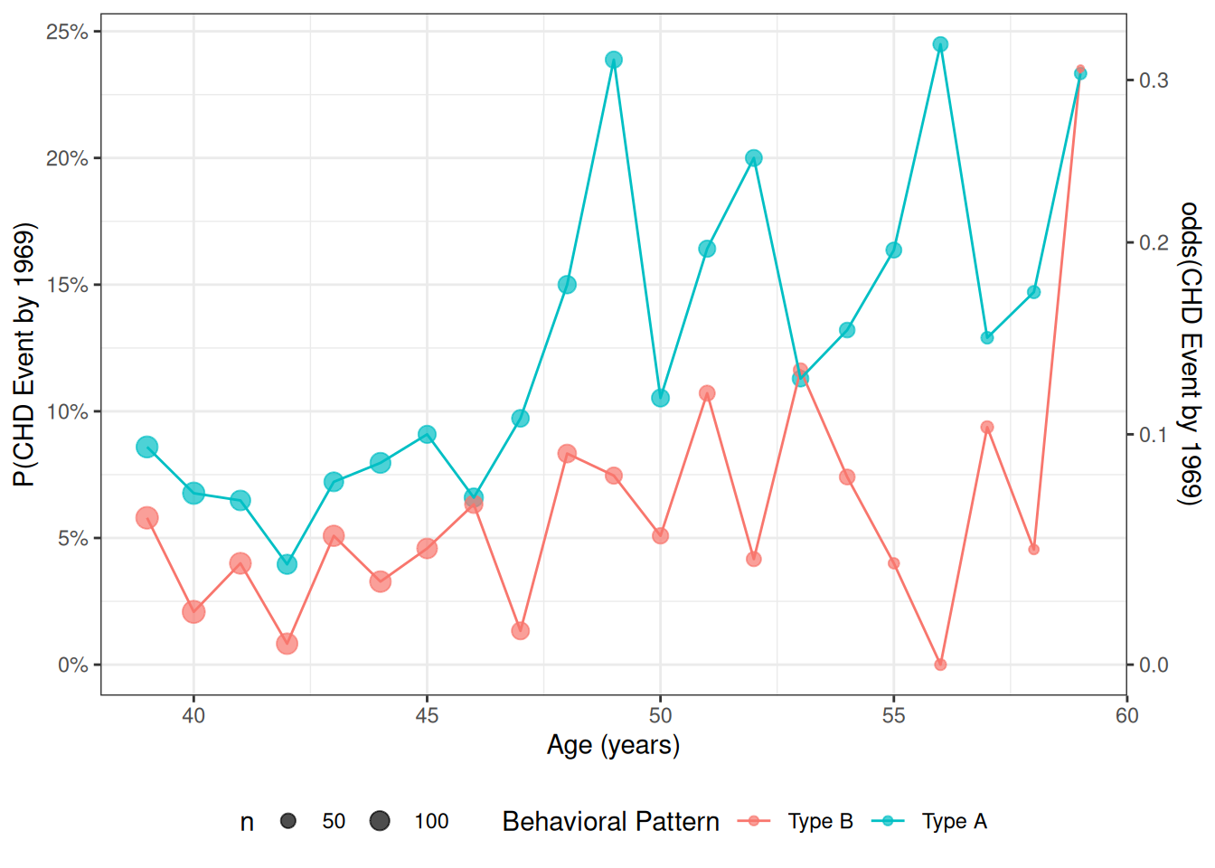
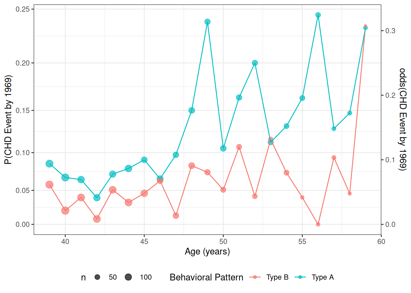
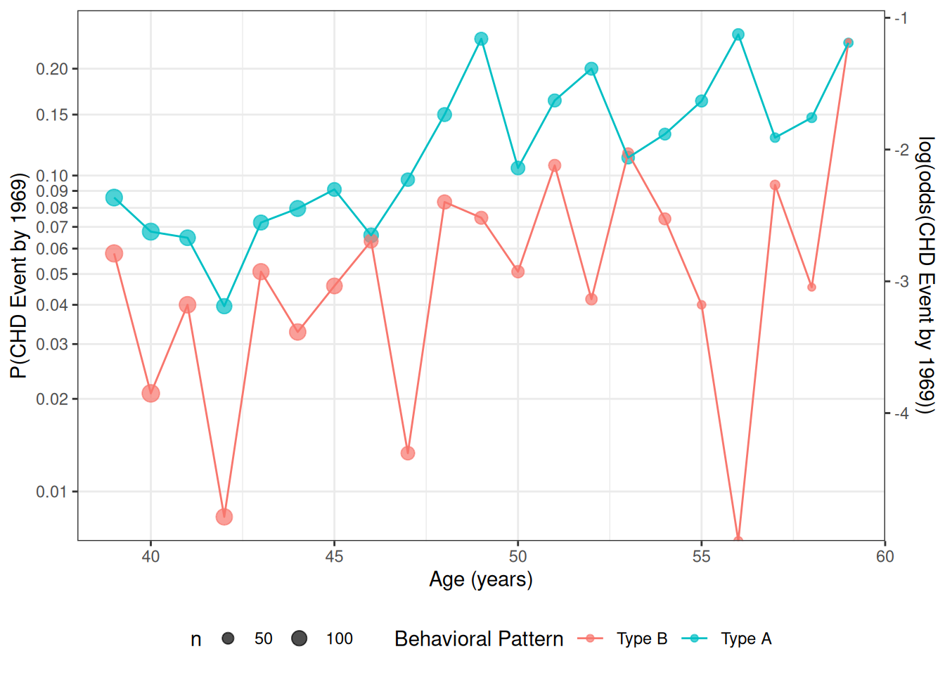
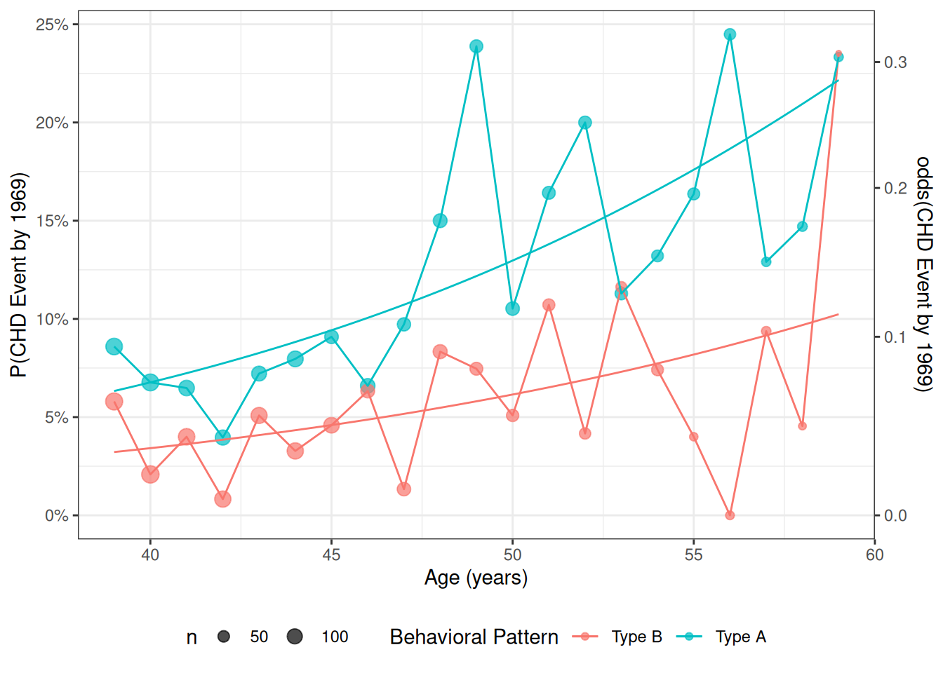
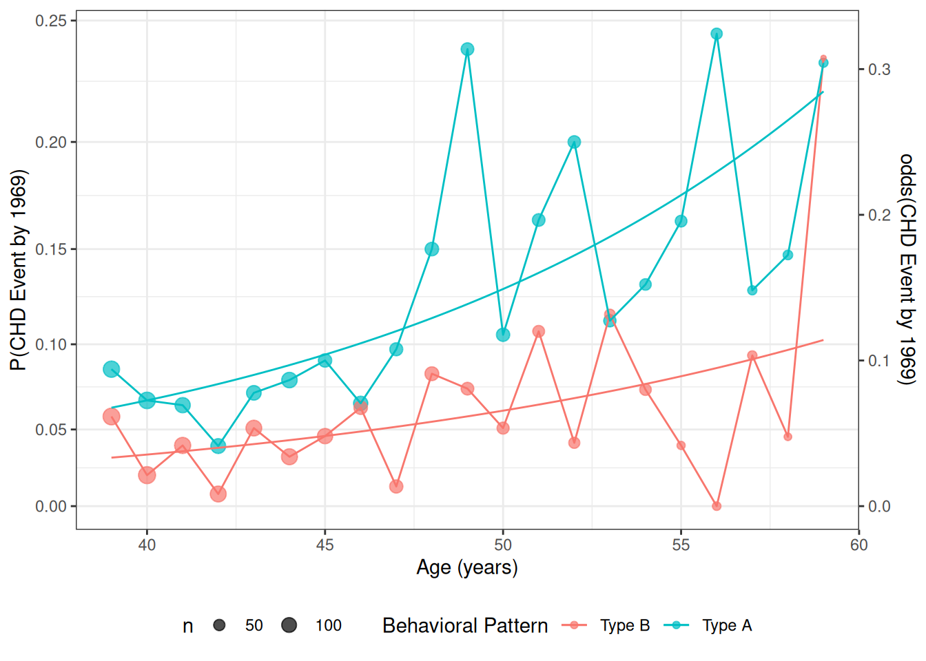
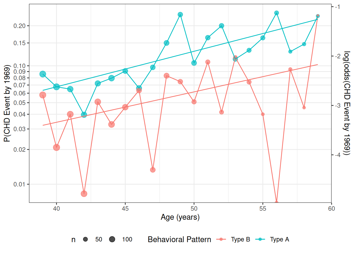
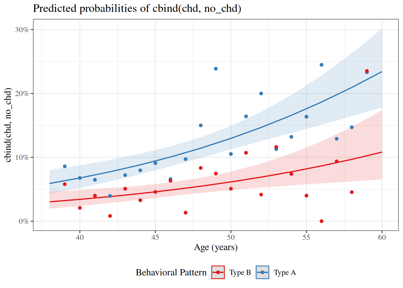
For now, we will look at the interaction between age and personality type (dibpat). To make it easier to visualize the data, we summarize the event rates for each combination of age:

library(dplyr)
odds <- function(pi) pi / (1 - pi)
chd_grouped_data <-
  wcgs |>
  summarize(
    .by = c(age, dibpat),
    n = sum(chd69 %in% c("Yes", "No")),
    x = sum(chd69 == "Yes")
  ) |>
  mutate(
    `n - x` = n - x,
    `p(chd)` = (x / n) |>
      labelled(label = "CHD Event by 1969"),
    `odds(chd)` = `p(chd)` / (1 - `p(chd)`),
    `logit(chd)` = log(`odds(chd)`)
  )

chd_grouped_data

Graphical exploration

library(ggplot2)
library(scales)
chd_plot_probs <-
  chd_grouped_data |>
  ggplot() +
  aes(
    x = age,
    y = `p(chd)`,
    col = dibpat
  ) +
  geom_point(aes(size = n), alpha = .7) +
  scale_size(range = c(1, 4)) +
  geom_line() +
  theme_bw() +
  ylab("P(CHD Event by 1969)") +
  scale_y_continuous(
    labels = scales::label_percent(),
    sec.axis = sec_axis(
      ~ odds(.),
      name = "odds(CHD Event by 1969)"
    )
  ) +
  theme(legend.position = "bottom")

print(chd_plot_probs)

Figure 11: CHD rates by age group, probability scale

7.1 Odds scale

odds_inv <- function(omega) omega / (1 + omega)
trans_odds <- trans_new(
  name = "odds",
  transform = odds,
  inverse = odds_inv
)

chd_plot_odds <- chd_plot_probs +
  scale_y_continuous(
    trans = trans_odds, # this line changes the vertical spacing
    name = chd_plot_probs$labels$y,
    sec.axis = sec_axis(
      ~ odds(.),
      name = "odds(CHD Event by 1969)"
    )
  )

print(chd_plot_odds)

Figure 12: CHD rates by age group, odds spacing

7.2 Log-odds (logit) scale

logit <- function(pi) log(odds(pi))
expit <- function(eta) odds_inv(exp(eta))
trans_logit <- trans_new(
  name = "logit",
  transform = logit,
  inverse = expit
)

chd_plot_logit <-
  chd_plot_probs +
  scale_y_continuous(
    trans = trans_logit, # this line changes the vertical spacing
    name = chd_plot_probs$labels$y,
    breaks = c(seq(.01, .1, by = .01), .15, .2),
    minor_breaks = NULL,
    sec.axis = sec_axis(
      ~ logit(.),
      name = "log(odds(CHD Event by 1969))"
    )
  )

print(chd_plot_logit)

Figure 13: CHD data (logit-scale)

Logistic regression models for CHD data

For the wcgs dataset, let’s consider a logistic regression model for the outcome of Coronary Heart Disease (\(Y\); chd in computer output):

• \(Y = 1\) if an individual developed CHD by the end of the study;
• \(Y = 0\) if they have not developed CHD by the end of the study.

Let’s include an intercept, two covariates, plus their interaction:

• \(A\): age at study enrollment (age, recorded in years)
• \(P\): personality type (dibpat):
  • \(P = 1\) represents “Type A personality”,
  • \(P = 0\) represents “Type B personality”.
• \(PA\): the interaction of personality type and age (dibpat:age)
• \(\tilde{X}= (1, A, P, PA)\)

chd_glm_contrasts <-
  wcgs |>
  glm(
    "data" = _,
    "formula" = chd69 == "Yes" ~ dibpat * age,
    "family" = binomial(link = "logit")
  )

library(equatiomatic)
equatiomatic::extract_eq(chd_glm_contrasts)

\[ \log\left[ \frac { P( \operatorname{chd69} = \operatorname{Yes} ) }{ 1 - P( \operatorname{chd69} = \operatorname{Yes} ) } \right] = \alpha + \beta_{1}(\operatorname{dibpat}_{\operatorname{Type\ A}}) + \beta_{2}(\operatorname{age}) + \beta_{3}(\operatorname{dibpat}_{\operatorname{Type\ A}} \times \operatorname{age}) \]

Or in more formal notation:

\[ \begin{aligned} Y_i | \tilde{X}_i &\ \sim_{\perp\!\!\!\perp}\ \operatorname{Ber}(\pi(\tilde{X}_i)) \\ \pi(\tilde{x}) &= \operatorname{expit}(\eta(\tilde{x})) \\ \eta(\tilde{x}) &= \beta_0 + \beta_P p + \beta_A a + \beta_{PA} pa \end{aligned} \tag{32}\]

Models superimposed on data

We can graph our fitted models on each scale (probability, odds, log-odds).

probability scale

curve_type_A <- function(x) { # nolint: object_name_linter
  chd_glm_contrasts |> predict(
    type = "response",
    newdata = tibble(age = x, dibpat = "Type A")
  )
}

curve_type_B <- function(x) { # nolint: object_name_linter
  chd_glm_contrasts |> predict(
    type = "response",
    newdata = tibble(age = x, dibpat = "Type B")
  )
}

chd_plot_probs_2 <-
  chd_plot_probs +
  geom_function(
    fun = curve_type_A,
    aes(col = "Type A")
  ) +
  geom_function(
    fun = curve_type_B,
    aes(col = "Type B")
  )
print(chd_plot_probs_2)

Figure 14: Fitted CHD risk by age and behavior pattern (probability scale)

odds scale

chd_plot_odds_2 <-
  chd_plot_odds +
  geom_function(
    fun = curve_type_A,
    aes(col = "Type A")
  ) +
  geom_function(
    fun = curve_type_B,
    aes(col = "Type B")
  )
print(chd_plot_odds_2)

Figure 15: Fitted CHD odds by age and behavior pattern (odds scale)

log-odds (logit) scale

chd_plot_logit_2 <-
  chd_plot_logit +
  geom_function(
    fun = curve_type_A,
    aes(col = "Type A")
  ) +
  geom_function(
    fun = curve_type_B,
    aes(col = "Type B")
  )

print(chd_plot_logit_2)

Figure 16: Fitted CHD log-odds by age and behavior pattern (log-odds scale)

Interpreting the model parameters

Exercise 25 For Equation 32, derive interpretations of \(\beta_0\), \(\beta_P\), \(\beta_A\), and \(\beta_{PA}\) on the odds and log-odds scales, State the interpretations concisely in math and in words.

(Hint: apply the general procedure for interpreting a regression coefficient to the log-odds linear predictor \(\eta(\tilde{x}) = \operatorname{logit}(\pi(\tilde{x}))\).)

Solution 25.  

# include: false
age_offset = 0L

\[ \begin{aligned} \eta(P=0,A=0) &= \beta_0 + \beta_P \cdot 0 + \beta_A \cdot 0 + \beta_{PA} (0 \cdot 0) && \text{(model equation, with } p = 0, a = 0 \text{)} \\ &= \beta_0 + 0 + 0 + 0 && \text{(multiplication by zero)} \\ &= \beta_0 && \text{(additive identity)} \end{aligned} \]

Therefore:

\[\beta_{0} = \eta(P=0,A=0) \tag{33}\]

\(\beta_{0}\) is the natural logarithm of the odds (“log-odds”) of experiencing CHD for a 0 year-old person with a type B personality; that is,

The WCGS cohort ranges in age from 39 to 59 years, so a 0-year-old is far outside the observed data. This intercept is therefore an extrapolation with no in-sample referent. Centering age at a representative value (replacing \(A\) with \(A - \bar{A}\)) is the standard remedy: it makes the intercept the log-odds at the mean age, which does have in-sample support.

---

\(\text{e}^{\beta_{0}}\) is the odds of experiencing CHD for a 0 year-old with a type B personality. Here we write

\[\omega(p, a) \stackrel{\text{def}}{=}\operatorname{odds}(Y=1|P=p, A=a)\]

for the odds of CHD at covariate values \((p, a)\). Then:

\[ \begin{aligned} \operatorname{exp}\mathopen{}\left\{\beta_{0}\right\}\mathclose{} &= \operatorname{exp}\mathopen{}\left\{\eta(P=0,A=0)\right\}\mathclose{} && \text{(} \beta_0 \text{ as a log-odds)} \\ &= \omega(P=0,A=0) && \text{(exponential of log-odds is odds: } \omega= \operatorname{exp}\mathopen{}\left\{\eta\right\}\mathclose{} \text{)} \\ &= \frac{\Pr(Y= 1| P = 0, A = 0)}{1-\Pr(Y= 1| P = 0, A = 0)} && \text{(definition of odds)} \\ &= \frac {\Pr(Y= 1| P = 0, A = 0)} {\Pr(Y= 0| P = 0, A = 0)} && \text{(complement rule: } 1 - \Pr(Y=1|\cdot) = \Pr(Y=0|\cdot) \text{)} \end{aligned} \]

As with the log-odds interpretation, this odds is evaluated at age 0, which lies outside the cohort’s 39-to-59-year age range, so \(\text{e}^{\beta_0}\) has no in-sample referent. Centering age before fitting gives an intercept whose odds is evaluated at the mean age instead.

---

\[ \begin{aligned} \frac{\partial}{\partial a}\eta(P=0, A = a) &= \frac{\partial}{\partial a} \mathopen{}\left(\beta_0 + \beta_P \cdot 0 + \beta_A a + \beta_{PA}(0\cdot a)\right)\mathclose{} && \text{(model equation, with } p = 0 \text{)} \\ &= \frac{\partial}{\partial a} \mathopen{}\left(\beta_0 + 0 + \beta_A a + 0\right)\mathclose{} && \text{(multiplication by zero)} \\ &= \frac{\partial}{\partial a} \mathopen{}\left(\beta_0 + \beta_A a\right)\mathclose{} && \text{(additive identity)} \\ &= \frac{\partial}{\partial a}\beta_0 + \frac{\partial}{\partial a}\mathopen{}\left(\beta_A a\right)\mathclose{} && \text{(linearity of differentiation)} \\ &= 0 + \beta_A && \text{(constants have derivative 0; derivative of a linear term)} \\ &= \beta_A && \text{(additive identity)} \end{aligned} \]

Therefore:

\[\beta_A = \frac{\partial}{\partial a}\eta(P=0, A = a) \tag{34}\]

\(\beta_A\) is the slope of the log-odds of CHD with respect to age, for individuals with personality type B.

Alternatively:

\[ \begin{aligned} \eta(P = 0, A = a + 1)- \eta(P = 0, A = a) &= \mathopen{}\left(\beta_0 + \beta_P \cdot 0 + \beta_A (a+1) + \beta_{PA} (0 \cdot (a+1))\right)\mathclose{} - \mathopen{}\left(\beta_0 + \beta_P \cdot 0 + \beta_A a + \beta_{PA} (0 \cdot a)\right)\mathclose{} && \text{(model equation, with } p = 0 \text{)} \\ &= \mathopen{}\left(\beta_0 + 0 + \beta_A (a+1) + 0\right)\mathclose{} - \mathopen{}\left(\beta_0 + 0 + \beta_A a + 0\right)\mathclose{} && \text{(multiplication by zero)} \\ &= \mathopen{}\left(\beta_0 + \beta_A (a+1)\right)\mathclose{} - \mathopen{}\left(\beta_0 + \beta_A a\right)\mathclose{} && \text{(additive identity)} \\ &= \beta_0 + \beta_A a + \beta_A - \beta_0 - \beta_A a && \text{(distribute)} \\ &= \beta_{A} && \text{(cancel } \beta_0 \text{ and } \beta_A a \text{)} \end{aligned} \]

That is, \(\beta_{A}\) is the difference in log-odds of experiencing CHD per one-year difference in age between two individuals with type B personalities.

---

\[ \begin{aligned} \operatorname{exp}\mathopen{}\left\{\beta_{A}\right\}\mathclose{} &= \operatorname{exp}\mathopen{}\left\{\eta(P = 0, A = a + 1)- \eta(P = 0, A = a)\right\}\mathclose{} && \text{(} \beta_A \text{ as a difference in log-odds)} \\ &= \frac{\operatorname{exp}\mathopen{}\left\{\eta(P = 0, A = a + 1)\right\}\mathclose{}}{\operatorname{exp}\mathopen{}\left\{\eta(P = 0, A = a)\right\}\mathclose{}} && \text{(exponential of a difference is a ratio)} \\ &= \frac{\omega(P = 0, A = a + 1)}{\omega(P = 0, A = a)} && \text{(exponential of log-odds is odds: } \omega= \operatorname{exp}\mathopen{}\left\{\eta\right\}\mathclose{} \text{)} \\ &= \frac {\operatorname{odds}(Y= 1|P=0, A = a + 1)} {\operatorname{odds}(Y= 1|P=0, A = a)} && \text{(the } \omega(p, a) \text{ notation defined at } \beta_0 \text{'s interpretation)} \\ &= \theta_{\omega}(\Delta a = 1 | P = 0) && \text{(definition of the odds ratio)} \end{aligned} \]

• The odds ratio of experiencing CHD (aka “the odds ratio”) differs by a factor of \(\text{e}^{\beta_{A}}\) per one-year difference in age between individuals with type B personality.

---

\(\beta_{P}\) is the difference in log-odds of experiencing CHD for a 0 year-old person with type A personality compared to a 0 year-old person with type B personality; that is,

\[\beta_P = \eta(P = 1, A = 0) - \eta(P=0, A = 0) \tag{35}\]

---

• \(\text{e}^{\beta_{P}}\) is the ratio of the odds (aka “the odds ratio”) of experiencing CHD, for a 0-year old individual with type A personality vs a 0-year old individual with type B personality; that is,

\[ \operatorname{exp}\mathopen{}\left\{\beta_{P}\right\}\mathclose{} = \frac {\operatorname{odds}(Y= 1|P=1, A = 0)} {\operatorname{odds}(Y= 1|P=0, A = 0)} \]

---

\[ \begin{aligned} \frac{\partial}{\partial a}\eta(P={\color{red}{1}}, A = a) &= \frac{\partial}{\partial a} \mathopen{}\left(\beta_0 + \beta_P \cdot 1 + \beta_A a + \beta_{PA}(1 \cdot a)\right)\mathclose{} && \text{(model equation, with } p = 1 \text{)} \\ &= \frac{\partial}{\partial a} \mathopen{}\left(\beta_0 + \beta_P + \beta_A a + \beta_{PA} a\right)\mathclose{} && \text{(multiplicative identity)} \\ &= \frac{\partial}{\partial a}\beta_0 + \frac{\partial}{\partial a}\beta_P + \frac{\partial}{\partial a}\mathopen{}\left(\beta_A a\right)\mathclose{} + \frac{\partial}{\partial a}\mathopen{}\left(\beta_{PA} a\right)\mathclose{} && \text{(linearity of differentiation)} \\ &= 0 + 0 + \beta_A + \beta_{PA} && \text{(constants have derivative 0; derivatives of linear terms)} \\ &= {\color{red}{\beta_A + \beta_{PA}}} && \text{(additive identity)} \\ \frac{\partial}{\partial a}\eta(P={\color{teal}{0}}, A = a) &= {\color{teal}{\beta_A}} && \text{(the type B slope, from the } \beta_A \text{ derivation)} \end{aligned} \]

Therefore:

\[ \begin{aligned} \frac{\partial}{\partial a}\eta(P={\color{red}{1}}, A = a) - \frac{\partial}{\partial a}\eta(P={\color{teal}{0}}, A = a) &= \mathopen{}\left({\color{red}{\beta_A + \beta_{PA}}}\right)\mathclose{} - {\color{teal}{\beta_A}} && \text{(substitute the two slopes)} \\ &= \beta_A - \beta_A + \beta_{PA} && \text{(commute the addition)} \\ &= \beta_{PA} && \text{(cancel } \beta_A \text{)} \end{aligned} \]

That is,

\[ \begin{aligned} \beta_{PA} &= \frac{\partial}{\partial a}\eta(P={\color{red}{1}}, A = a) - \frac{\partial}{\partial a}\eta(P={\color{teal}{0}}, A = a) && \text{(rearrange the difference of slopes)} \\ &= \frac{\partial}{\partial a}\eta(P={\color{red}{1}}, A = a) - {\color{teal}{\beta_A}} && \text{(substitute the type B slope, } \frac{\partial}{\partial a}\eta(P=0, A=a) = \beta_A \text{)} \end{aligned} \]

\(\beta_{PA}\) is the difference in the slopes of log-odds over age between participants with Type A personalities and participants with Type B personalities.

---

Accordingly, the odds ratio of experiencing CHD per one-year difference in age differs by a factor of \(\text{e}^{\beta_{PA}}\) for participants with type A personality compared to participants with type B personality; that is,

\[ \begin{aligned} \theta_{\omega}(\Delta a = 1 | P = 1) = \operatorname{exp}\mathopen{}\left\{\beta_{PA}\right\}\mathclose{} \times \theta_{\omega}(\Delta a = 1 | P = 0) \end{aligned} \]

or equivalently:

\[ \operatorname{exp}\mathopen{}\left\{\beta_{PA}\right\}\mathclose{} = \frac {\theta_{\omega}(\Delta a = 1 | P = 1)} {\theta_{\omega}(\Delta a = 1 | P = 0)} \]

See Section 5.1.1 of Vittinghoff et al. (2012) for another perspective, also using the wcgs data as an example.

Interpreting the model parameter estimates

Table 17 shows the fitted model.

library(parameters)
chd_glm_contrasts |>
  parameters() |>
  print_md()

Table 17: CHD model (corner-point parametrization)

Parameter	Log-Odds	SE	95% CI	z	p
(Intercept)	-5.80	0.98	(-7.73, -3.90)	-5.95	< .001
dibpat (Type A)	0.30	1.18	(-2.02, 2.63)	0.26	0.797
age	0.06	0.02	(0.02, 0.10)	3.01	0.003
dibpat (Type A) × age	0.01	0.02	(-0.04, 0.06)	0.42	0.674

We can get the corresponding odds ratio estimates (\(e^{\hat{\beta}}\)s) by passing exponentiate = TRUE to parameters():

chd_glm_contrasts |>
  parameters(exponentiate = TRUE) |>
  print_md()

Table 18: Odds ratio estimates for CHD model

Parameter	Odds Ratio	SE	95% CI	z	p
(Intercept)	3.02e-03	2.94e-03	(4.40e-04, 0.02)	-5.95	< .001
dibpat (Type A)	1.36	1.61	(0.13, 13.88)	0.26	0.797
age	1.06	0.02	(1.02, 1.11)	3.01	0.003
dibpat (Type A) × age	1.01	0.02	(0.96, 1.06)	0.42	0.674

Stratified parametrization

We could instead use a stratified parametrization:

chd_glm_strat <- glm(
  "formula" = chd69 == "Yes" ~ dibpat + dibpat:age - 1,
  "data" = wcgs,
  "family" = binomial(link = "logit")
)
equatiomatic::extract_eq(chd_glm_strat)

\[ \log\left[ \frac { P( \operatorname{chd69} = \operatorname{Yes} ) }{ 1 - P( \operatorname{chd69} = \operatorname{Yes} ) } \right] = \beta_{1}(\operatorname{dibpat}_{\operatorname{Type\ B}}) + \beta_{2}(\operatorname{dibpat}_{\operatorname{Type\ A}}) + \beta_{3}(\operatorname{dibpat}_{\operatorname{Type\ B}} \times \operatorname{dibpat}_{\operatorname{age}}) + \beta_{4}(\operatorname{dibpat}_{\operatorname{Type\ A}} \times \operatorname{dibpat}_{\operatorname{age}}) \]

chd_glm_strat |>
  parameters() |>
  print_md()

Table 19: CHD model, stratified parametrization

Parameter	Log-Odds	SE	95% CI	z	p
dibpat (Type B)	-5.80	0.98	(-7.73, -3.90)	-5.95	< .001
dibpat (Type A)	-5.50	0.67	(-6.83, -4.19)	-8.18	< .001
dibpat (Type B) × age	0.06	0.02	(0.02, 0.10)	3.01	0.003
dibpat (Type A) × age	0.07	0.01	(0.05, 0.10)	5.24	< .001

Again, we can get the corresponding odds ratios (\(e^{\beta}\)s) by passing exponentiate = TRUE to parameters():

chd_glm_strat |>
  parameters(exponentiate = TRUE) |>
  print_md()

Table 20: Odds ratio estimates for CHD model

Parameter	Odds Ratio	SE	95% CI	z	p
dibpat (Type B)	3.02e-03	2.94e-03	(4.40e-04, 0.02)	-5.95	< .001
dibpat (Type A)	4.09e-03	2.75e-03	(1.08e-03, 0.02)	-8.18	< .001
dibpat (Type B) × age	1.06	0.02	(1.02, 1.11)	3.01	0.003
dibpat (Type A) × age	1.07	0.01	(1.05, 1.10)	5.24	< .001

Compare with Table 17.

Exercise 26 If I give you model 1, how would you get the coefficients of model 2?

Solution 26. Model 1 is the corner-point (reference/contrast) parametrization fitted in chd_glm_contrasts, with linear predictor (Equation 32):

\[\eta(p, a) = \beta_0 + \beta_P p + \beta_A a + \beta_{PA} pa\]

Model 2 is the stratified parametrization fitted in chd_glm_strat, which gives each personality type its own intercept and its own age slope. Writing \(\gamma_B, \gamma_A\) for the stratum-specific intercepts and \(\delta_B, \delta_A\) for the stratum-specific age slopes:

\[ \eta(p, a) \stackrel{\text{def}}{=} \gamma_B (1 - p) + \gamma_A p + \delta_B (1 - p) a + \delta_A p a \tag{36}\]

The two parametrizations span the same set of linear-predictor functions, so both models have the same fitted linear predictor \(\eta(p, a)\). We can therefore recover the model 2 coefficients by equating the two expressions for \(\eta(p, a)\) within each personality-type stratum.

---

Type B stratum (\(p = 0\)):

In model 1 (Equation 32):

\[ \begin{aligned} \eta(0, a) &= \beta_0 + \beta_P \cdot 0 + \beta_A a + \beta_{PA} \cdot 0 \cdot a && \text{(substitute } p = 0\text{)} \\ &= \beta_0 + 0 + \beta_A a + 0 && \text{(multiply by 0)} \\ &= \beta_0 + \beta_A a && \text{(drop the zero terms)} \end{aligned} \]

In model 2 (Equation 36):

\[ \begin{aligned} \eta(0, a) &= \gamma_B (1 - 0) + \gamma_A \cdot 0 + \delta_B (1 - 0) a + \delta_A \cdot 0 \cdot a && \text{(substitute } p = 0\text{)} \\ &= \gamma_B \cdot 1 + \gamma_A \cdot 0 + \delta_B \cdot 1 \cdot a + \delta_A \cdot 0 \cdot a && \text{(} 1 - 0 = 1 \text{)} \\ &= \gamma_B + 0 + \delta_B a + 0 && \text{(multiply by 1 and by 0)} \\ &= \gamma_B + \delta_B a && \text{(drop the zero terms)} \end{aligned} \]

---

Equating the two expressions for \(\eta(0, a)\), for all ages \(a\):

\[ \gamma_B + \delta_B a = \beta_0 + \beta_A a \tag{37}\]

Setting \(a = 0\) in Equation 37:

\[ \begin{aligned} \gamma_B + \delta_B \cdot 0 &= \beta_0 + \beta_A \cdot 0 && \text{(substitute } a = 0\text{)} \\ \gamma_B + 0 &= \beta_0 + 0 && \text{(multiply by 0)} \\ \gamma_B &= \beta_0 && \text{(drop the zero terms)} \end{aligned} \]

Subtracting \(\gamma_B = \beta_0\) from both sides of Equation 37 and then setting \(a = 1\):

\[ \begin{aligned} \delta_B a &= \beta_A a && \text{(subtract } \gamma_B = \beta_0 \text{ from both sides)} \\ \delta_B \cdot 1 &= \beta_A \cdot 1 && \text{(substitute } a = 1\text{)} \\ \delta_B &= \beta_A && \text{(multiply by 1)} \end{aligned} \]

---

Type A stratum (\(p = 1\)):

In model 1 (Equation 32):

\[ \begin{aligned} \eta(1, a) &= \beta_0 + \beta_P \cdot 1 + \beta_A a + \beta_{PA} \cdot 1 \cdot a && \text{(substitute } p = 1\text{)} \\ &= \beta_0 + \beta_P + \beta_A a + \beta_{PA} a && \text{(multiply by 1)} \\ &= (\beta_0 + \beta_P) + (\beta_A + \beta_{PA}) a && \text{(group the constant terms; factor out } a \text{)} \end{aligned} \]

In model 2 (Equation 36):

\[ \begin{aligned} \eta(1, a) &= \gamma_B (1 - 1) + \gamma_A \cdot 1 + \delta_B (1 - 1) a + \delta_A \cdot 1 \cdot a && \text{(substitute } p = 1\text{)} \\ &= \gamma_B \cdot 0 + \gamma_A \cdot 1 + \delta_B \cdot 0 \cdot a + \delta_A \cdot 1 \cdot a && \text{(} 1 - 1 = 0 \text{)} \\ &= 0 + \gamma_A + 0 + \delta_A a && \text{(multiply by 0 and by 1)} \\ &= \gamma_A + \delta_A a && \text{(drop the zero terms)} \end{aligned} \]

Equating the two expressions for \(\eta(1, a)\) and applying the same two steps as in the Type B stratum (set \(a = 0\); then subtract the intercepts and set \(a = 1\)):

\[ \begin{aligned} \gamma_A &= \beta_0 + \beta_P \\ \delta_A &= \beta_A + \beta_{PA} \end{aligned} \]

---

Summary of the conversion:

\[ \begin{aligned} \gamma_B &= \beta_0 \\ \gamma_A &= \beta_0 + \beta_P \\ \delta_B &= \beta_A \\ \delta_A &= \beta_A + \beta_{PA} \end{aligned} \tag{38}\]

Solving Equation 38 for the model 1 coefficients inverts the conversion, so either parametrization determines the other:

\[ \begin{aligned} \beta_0 &= \gamma_B && \text{(first equation of the summary)} \\ \beta_P &= \gamma_A - \gamma_B && \text{(subtract the first equation from the second)} \\ \beta_A &= \delta_B && \text{(third equation)} \\ \beta_{PA} &= \delta_A - \delta_B && \text{(subtract the third equation from the fourth)} \end{aligned} \]

---

Numerical check: applying Equation 38 to the fitted model 1 coefficients (Table 17) reproduces the fitted model 2 coefficients (Table 19):

b <- coef(chd_glm_contrasts)

gamma_delta <- c(
  "dibpatType B" = unname(b["(Intercept)"]),
  "dibpatType A" = unname(b["(Intercept)"] + b["dibpatType A"]),
  "dibpatType B:age" = unname(b["age"]),
  "dibpatType A:age" = unname(b["age"] + b["dibpatType A:age"])
)

cbind(
  "converted from model 1" = gamma_delta,
  "model 2 (fitted directly)" = coef(chd_glm_strat)[names(gamma_delta)]
)
#>                  converted from model 1 model 2 (fitted directly)
#> dibpatType B                 -5.8032532                -5.8032532
#> dibpatType A                 -5.4988618                -5.4988618
#> dibpatType B:age              0.0615634                 0.0615634
#> dibpatType A:age              0.0719071                 0.0719071

8 Model comparisons for logistic models

Deviance test

Definition 4 (Deviance goodness-of-fit test) We can compare the maximized log-likelihood of our model, \(\ell(\hat\beta; \mathbf x)\), versus the log-likelihood of the full model (aka saturated model aka maximal model), \(\ell_{\text{full}}\), which has one parameter per covariate pattern. The deviance statistic is:

\[D \stackrel{\text{def}}{=}2(\ell_{\text{full}} - \ell(\hat\beta; \mathbf x))\]

With enough data, \(D \dot \sim \chi^2(q - p)\), where \(q\) is the number of distinct covariate patterns and \(p\) is the number of \(\beta\) parameters in our model. The deviance test compares \(D\) to that \(\chi^2(q-p)\) distribution; a significant p-value for this deviance statistic indicates that there’s some detectable pattern in the data that our model isn’t flexible enough to catch.

Caution

The deviance statistic needs to have a large amount of data for each covariate pattern for the \(\chi^2\) approximation to hold. A guideline from Dobson and Barnett (2018, chap. 5) is that if there are \(q\) distinct covariate patterns \(x_1...,x_q\), with \(n_1,...,n_q\) observations per pattern, then the expected frequencies \(n_k \cdot \pi(x_k)\) should be at least 1 for every pattern \(k\in 1:q\).

If you have covariates measured on a continuous scale, you may not be able to use the deviance tests to assess goodness of fit.

Example 6 (Deviance test for the WCGS CHD model) Our CHD model chd_glm_contrasts was fit to individual-level observations, but its covariate patterns are just the combinations of personality type (dibpat) and whole-year age, so we can refit the same model to the grouped data and perform the deviance test:

wcgs_gof_grouped <-
  wcgs |>
  summarize(
    .by = c(dibpat, age),
    n = n(),
    chd = sum(chd69 == "Yes"),
    no_chd = sum(chd69 == "No")
  )

chd_glm_gof_grouped <- glm(
  "formula" = cbind(chd, no_chd) ~ dibpat * age,
  "data" = wcgs_gof_grouped,
  "family" = binomial(link = "logit")
)

deviance_gof <- deviance(chd_glm_gof_grouped)
q_gof <- nrow(wcgs_gof_grouped)
p_gof <- length(coef(chd_glm_gof_grouped))
pval_deviance_gof <- pchisq(
  deviance_gof,
  df = q_gof - p_gof,
  lower.tail = FALSE
)
min_exp_freq <- min(wcgs_gof_grouped$n * fitted(chd_glm_gof_grouped))

The smallest expected event frequency across the covariate patterns is \(\min_k \left\{ n_k \cdot \hat\pi(x_k) \right\} = 1.74\), which is at least 1, so these grouped data meet the minimum-expected-frequency guideline from Dobson and Barnett (2018, chap. 5) for using the \(\chi^2\) approximation.

The grouped data have \(q = 42\) distinct covariate patterns, and the model has \(p = 4\) parameters, so the deviance statistic \(D = 45\) has \(q - p = 38\) degrees of freedom. The corresponding p-value is \(p(\chi^2(38) > 45) = 0.202\), so the deviance test finds no significant evidence of lack of fit for this model.

Hosmer-Lemeshow test

If our covariate patterns produce groups that are too small, a reasonable solution is to make bigger groups by merging some of the covariate-pattern groups together.

Definition 5 (Hosmer-Lemeshow test) Hosmer and Lemeshow (1980) proposed that we group the patterns by their predicted probabilities according to the model of interest. For example, you could group all of the observations with predicted probabilities of 10% or less together, then group the observations with 11%-20% probability together, and so on; \(g=10\) categories in all.

Then we can construct a statistic \[X^2 \stackrel{\text{def}}{=}\sum_{c=1}^g \frac{(o_c - e_c)^2}{e_c}\] where \(o_c\) is the number of events observed in group \(c\), and \(e_c\) is the number of events expected in group \(c\) (based on the sum of the fitted values \(\hat\pi_i\) for observations in group \(c\)).

If each group has enough observations in it, you can compare \(X^2\) to a \(\chi^2\) distribution; by simulation, the degrees of freedom has been found to be approximately \(g-2\).

Note

The Hosmer-Lemeshow statistic depends on how the observations are grouped. Changing the number of groups \(g\), or the cut points used to form them, can change the value of \(X^2\) and its p-value for the same fitted model, so the test can reach different conclusions depending on the grouping choice. Hosmer et al. (1997) compare the Hosmer-Lemeshow test against several alternative goodness-of-fit tests and document this sensitivity.

Example 7 (Hosmer-Lemeshow test for the WCGS CHD model) For our CHD model, this procedure would be:

wcgs <-
  wcgs |>
  mutate(
    pred_probs_glm1 = chd_glm_contrasts |> fitted(),
    pred_prob_cats1 = pred_probs_glm1 |>
      cut(
        breaks = seq(0, 1, by = .1),
        include.lowest = TRUE
      )
  )

HL_table <- # nolint: object_name_linter
  wcgs |>
  summarize(
    .by = pred_prob_cats1,
    n = n(),
    o = sum(chd69 == "Yes"),
    e = sum(pred_probs_glm1)
  )

library(pander)
HL_table |> pander()

pred_prob_cats1	n	o	e
(0.1,0.2]	785	116	108
(0.2,0.3]	64	12	13.77
[0,0.1]	2,305	129	135.2

X2 <- HL_table |> # nolint: object_name_linter
  summarize(
    `X^2` = sum((o - e)^2 / e)
  ) |>
  pull(`X^2`)
print(X2)
#> [1] 1.11029

pval1 <- pchisq(X2, lower = FALSE, df = nrow(HL_table) - 2)

Our statistic is \(X^2 = 1.110287\); \(p(\chi^2(1) > 1.110287) = 0.29202\), which is our p-value for detecting a lack of goodness of fit.

Unfortunately that grouping plan left us with just three categories with any observations, so instead of grouping by 10% increments of predicted probability, typically analysts use deciles of the predicted probabilities:

wcgs <-
  wcgs |>
  mutate(
    pred_probs_glm1 = chd_glm_contrasts |> fitted(),
    pred_prob_cats1 = pred_probs_glm1 |>
      cut(
        breaks = quantile(pred_probs_glm1, seq(0, 1, by = .1)),
        include.lowest = TRUE
      )
  )

HL_table <- # nolint: object_name_linter
  wcgs |>
  summarize(
    .by = pred_prob_cats1,
    n = n(),
    o = sum(chd69 == "Yes"),
    e = sum(pred_probs_glm1)
  )

HL_table |> pander()

pred_prob_cats1	n	o	e
(0.114,0.147]	275	48	36.81
(0.147,0.222]	314	51	57.19
(0.0774,0.0942]	371	27	32.56
(0.0942,0.114]	282	30	29.89
(0.0633,0.069]	237	17	15.97
(0.069,0.0774]	306	20	22.95
(0.0487,0.0633]	413	27	24.1
(0.0409,0.0487]	310	14	14.15
[0.0322,0.0363]	407	16	13.91
(0.0363,0.0409]	239	7	9.48

X2 <- HL_table |> # nolint: object_name_linter
  summarize(
    `X^2` = sum((o - e)^2 / e)
  ) |>
  pull(`X^2`)

print(X2)
#> [1] 6.78114

pval1 <- pchisq(X2, lower = FALSE, df = nrow(HL_table) - 2)

Now we have more evenly split categories. The p-value is \(0.56042\), still not significant.

Graphically, we have compared:

HL_plot <- # nolint: object_name_linter
  HL_table |>
  ggplot(aes(x = pred_prob_cats1)) +
  geom_line(
    aes(y = e, x = pred_prob_cats1, group = "Expected", col = "Expected")
  ) +
  geom_point(aes(y = e, size = n, col = "Expected")) +
  geom_point(aes(y = o, size = n, col = "Observed")) +
  geom_line(aes(y = o, col = "Observed", group = "Observed")) +
  scale_size(range = c(1, 4)) +
  theme_bw() +
  ylab("number of CHD events") +
  theme(axis.text.x = element_text(angle = 45))

ggplotly(HL_plot)

Comparing models

The deviance test (Definition 4) and the Hosmer-Lemeshow test (Definition 5) assess the fit of a single model in absolute terms. To choose between two competing models, we can instead compare their fits against each other, using criteria that trade off fit against complexity:

• AIC = \(-2 * \ell(\hat\theta) + 2 * p\) [lower is better] (Akaike 1974) (see the AIC definition)
• BIC = \(-2 * \ell(\hat\theta) + p * \text{log}(n)\) [lower is better] (Schwarz 1978) (see the BIC definition)

A larger maximized log-likelihood is not, by itself, evidence that one model is better than another: adding parameters to a model can never decrease its maximized log-likelihood, so the more complex of two nested models always fits at least as well. For nested models, the likelihood ratio test accounts for this complexity difference by testing whether the improvement in fit is larger than chance alone would produce:

Definition 6 (Likelihood ratio test (LRT)) Suppose a reduced model with \(p_0\) parameters is nested in a full model with \(p_1 > p_0\) parameters; that is, the reduced model is a special case of the full model. The likelihood ratio test statistic is:

\[\Lambda \stackrel{\text{def}}{=}2(\ell_{\text{full}}(\hat\theta_1) - \ell_{\text{red}}(\hat\theta_0))\]

where \(\hat\theta_1\) and \(\hat\theta_0\) are the maximum likelihood estimates of the full and reduced models, respectively. Under the null hypothesis that the reduced model is adequate, \(\Lambda \dot \sim \chi^2(p_1 - p_0)\) by Wilks’ theorem. The likelihood ratio test (LRT) rejects the reduced model when \(\Lambda\) is large relative to that \(\chi^2(p_1 - p_0)\) distribution.

See also the likelihood ratio test for linear models.

Example 8 (Testing the WCGS interaction term with a likelihood ratio test) Our CHD model chd_glm_contrasts includes a dibpat:age interaction term. Does that interaction term improve the fit enough to justify its extra parameter? Let’s fit the nested model without the interaction term and compare the two models with a likelihood ratio test:

chd_glm_additive <-
  wcgs |>
  glm(
    "data" = _,
    "formula" = chd69 == "Yes" ~ dibpat + age,
    "family" = binomial(link = "logit")
  )

lrt_chd <- anova(
  chd_glm_additive,
  chd_glm_contrasts,
  test = "LRT"
)
lrt_chd

llik_full_chd <- logLik(chd_glm_contrasts) |> as.numeric()
llik_red_chd <- logLik(chd_glm_additive) |> as.numeric()
lambda_chd <- lrt_chd$Deviance[2]
df_chd <- lrt_chd$Df[2]
pval_lrt_chd <- lrt_chd$`Pr(>Chi)`[2]

Here the test statistic is:

\[ \begin{aligned} \Lambda &\stackrel{\text{def}}{=}2(\ell_{\text{full}}(\hat\theta_1) - \ell_{\text{red}}(\hat\theta_0)) && \text{(definition of the LRT statistic)} \\ &= 2 \times (-851.99 - (-852.08)) && \text{(substituting the two maximized log-likelihoods)} \\ &= 2 \times 0.09 && \text{(subtraction)} \\ &= 0.18 && \text{(multiplication)} \end{aligned} \]

The full model has \(p_1 = 4\) parameters and the reduced model has \(p_0 = 3\), so the null distribution is \(\chi^2(p_1 - p_0) = \chi^2(1)\), and the p-value is \(p(\chi^2(1) > 0.18) = 0.674\). The LRT finds no significant evidence that the interaction term improves the fit.

The lrtest() function from the {lmtest} package performs the same test:

lmtest::lrtest(chd_glm_contrasts, chd_glm_additive)

AIC and BIC can also compare these two models:

AIC(chd_glm_additive, chd_glm_contrasts)

BIC(chd_glm_additive, chd_glm_contrasts)

Both criteria are lower for the additive model (AIC: \(1710.16\) vs \(1711.98\); BIC: \(1728.33\) vs \(1736.21\)), agreeing with the LRT that the interaction term is not worth its extra parameter.

9 Residual-based diagnostics

Logistic regression residuals only work for grouped data

The residual and leverage diagnostics in this section follow the logistic-regression diagnostics developed by Pregibon (1981); see also Dobson and Barnett (2018, chap. 7) and Vittinghoff et al. (2012, chap. 5) for textbook treatments.

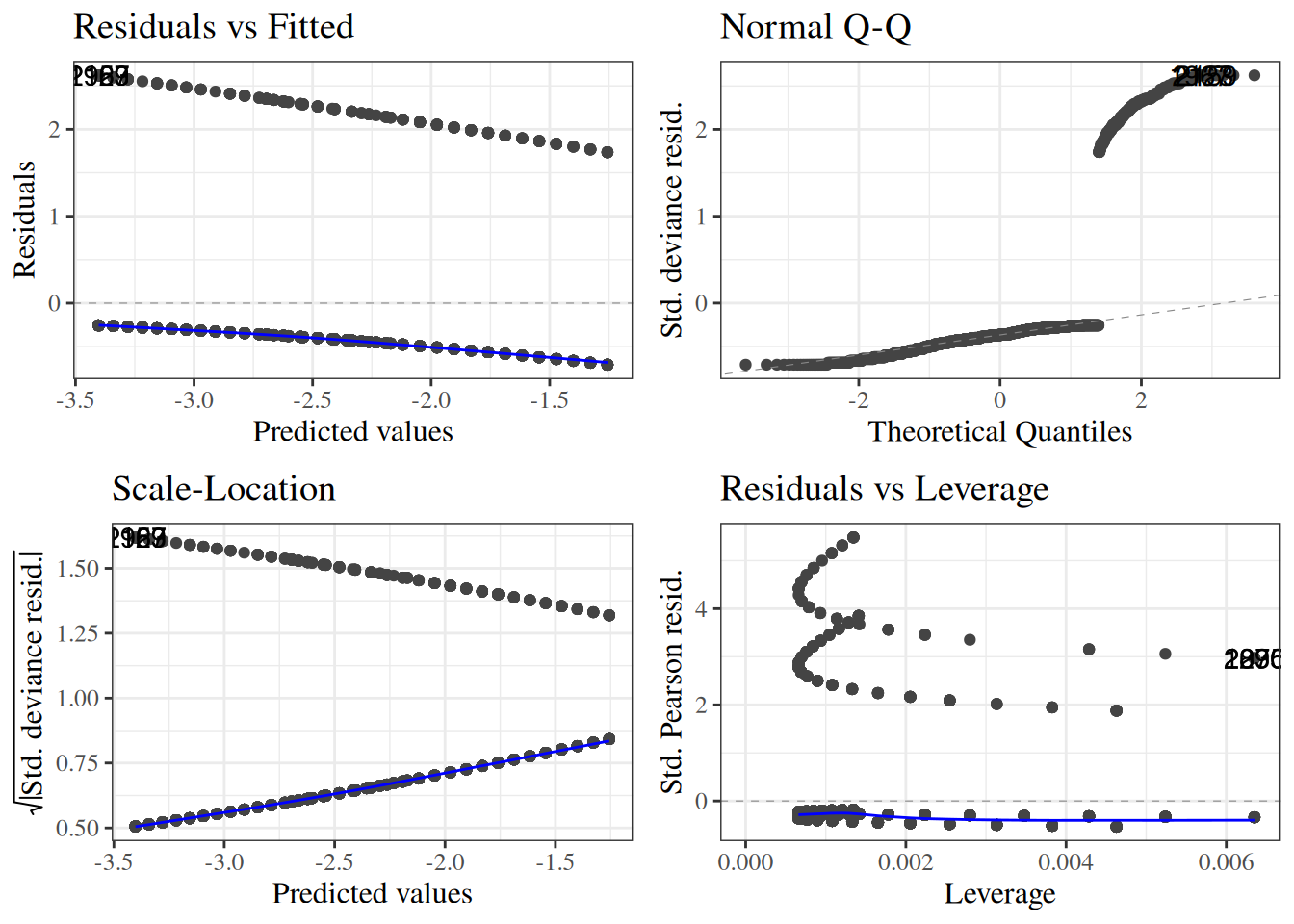
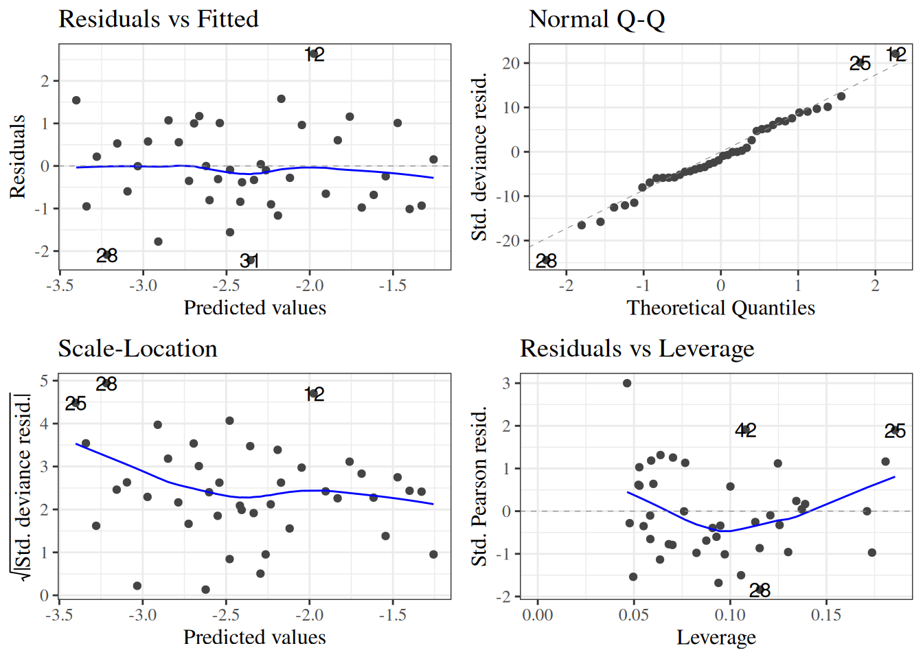
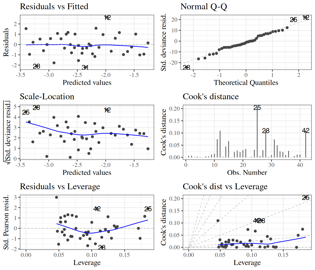
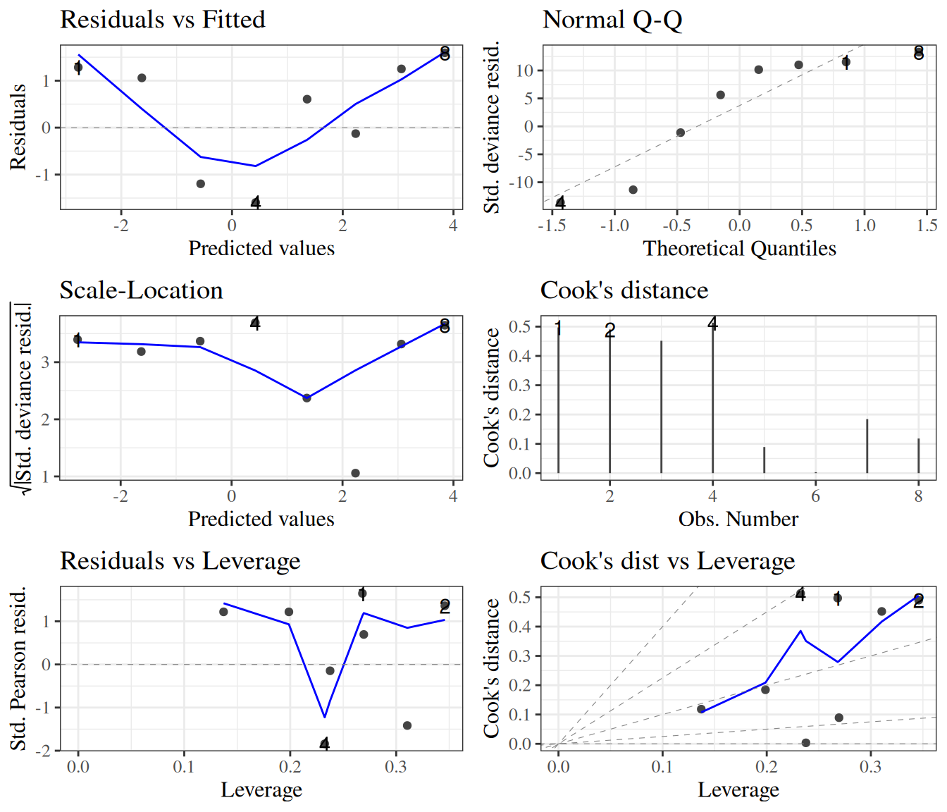
library(haven)
url <- paste0(
  # I'm breaking up the url into two chunks for readability
  "https://regression.ucsf.edu/sites/g/files/",
  "tkssra6706/f/wysiwyg/home/data/wcgs.dta"
)
library(here) # provides the `here()` function
library(fs) # provides the `path()` function
here::here() |>
  fs::path("Data/wcgs.rda") |>
  load()
chd_glm_contrasts <-
  wcgs |>
  glm(
    "data" = _,
    "formula" = chd69 == "Yes" ~ dibpat * age,
    "family" = binomial(link = "logit")
  )
library(ggfortify)
chd_glm_contrasts |> autoplot()

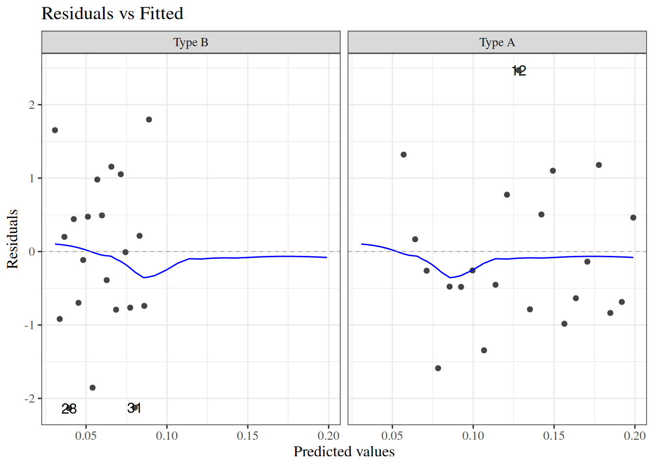
Figure 17: Residual diagnostics for WCGS model with individual-level observations

Residuals only work if there is more than one observation for most covariate patterns.

Here we will create the grouped-data version of our CHD model from the WCGS study:

library(dplyr)
wcgs_grouped <-
  wcgs |>
  summarize(
    .by = c(dibpat, age),
    n = n(),
    chd = sum(chd69 == "Yes"),
    no_chd = sum(chd69 == "No")
  ) |> 
  mutate(p_chd = chd/n)

chd_glm_contrasts_grouped <- glm(
  "formula" = cbind(chd, no_chd) ~ dibpat*age,
  "data" = wcgs_grouped,
  "family" = binomial(link = "logit")
)
chd_glm_contrasts_grouped |> equatiomatic::extract_eq()

\[ \log\left[ \frac { P( \operatorname{chd} ) }{ 1 - P( \operatorname{chd} ) } \right] = \alpha + \beta_{1}(\operatorname{dibpat}_{\operatorname{Type\ A}}) + \beta_{2}(\operatorname{age}) + \beta_{3}(\operatorname{dibpat}_{\operatorname{Type\ A}} \times \operatorname{age}) \]

library(parameters)
chd_glm_contrasts_grouped |>
  parameters() |>
  print_md()

Table 21: CHD model with grouped wcgs data

Parameter	Log-Odds	SE	95% CI	z	p
(Intercept)	-5.80	0.98	(-7.73, -3.90)	-5.95	< .001
dibpat (Type A)	0.30	1.18	(-2.02, 2.63)	0.26	0.797
age	0.06	0.02	(0.02, 0.10)	3.01	0.003
dibpat (Type A) × age	0.01	0.02	(-0.04, 0.06)	0.42	0.674

chd_glm_contrasts_grouped |> 
  sjPlot::plot_model(type = "pred", terms = c("age", "dibpat")) + 
  geom_point(data = wcgs_grouped |> mutate(group_col = dibpat), 
             aes(x = age, y = p_chd))

Figure 18: CHD model with grouped wcgs data

library(ggfortify)
chd_glm_contrasts_grouped |> autoplot()

(Response) residuals

Definition 7  

Response residual

The response residual for covariate pattern \(k\) is

\[e_k \stackrel{\text{def}}{=}\bar y_k - \hat{\pi}(x_k)\]

where \(k\) indexes the covariate patterns, \(\bar y_k\) is the observed proportion of events in pattern \(k\), and \(\hat\pi(x_k)\) is the fitted probability for pattern \(k\).

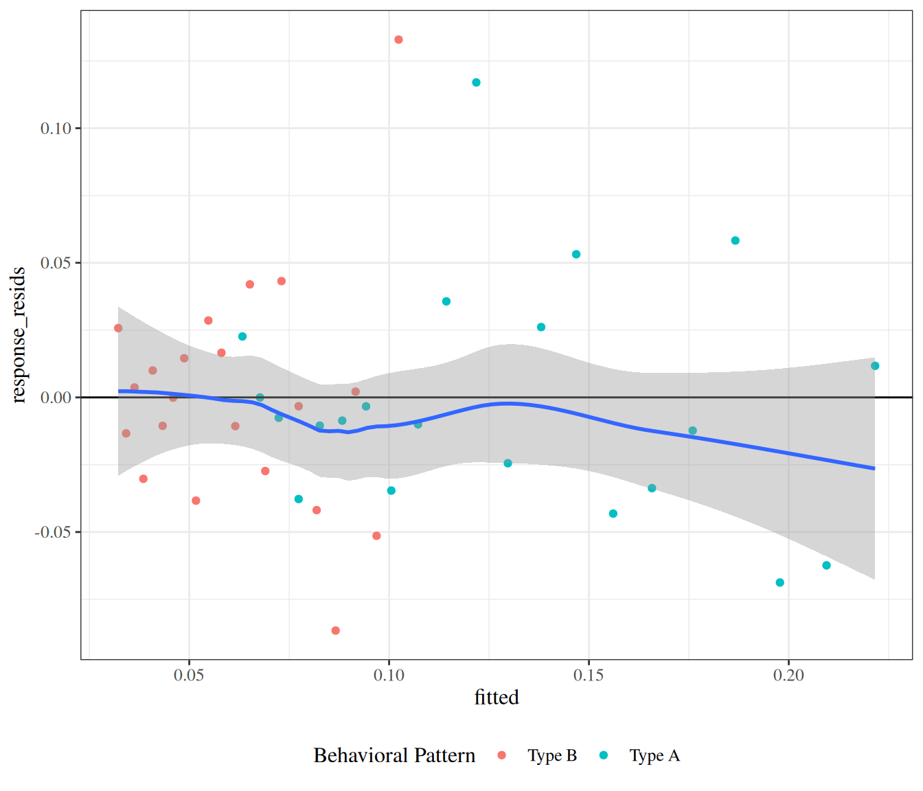
Example 9 (Response residuals for the WCGS CHD model) We can graph these residuals \(e_k\) (Definition 7) against the fitted values \(\hat\pi(x_k)\):

odds <- function(pi) pi/(1-pi)
logit <- function(pi) log(odds(pi))
wcgs_grouped <-
  wcgs_grouped |>
  mutate(
    fitted = chd_glm_contrasts_grouped |> fitted(),
    fitted_logit = fitted |> logit(),
    response_resids = chd_glm_contrasts_grouped |> resid(type = "response")
  )

wcgs_response_resid_plot <-
  wcgs_grouped |>
  ggplot(
    mapping = aes(
      x = fitted,
      y = response_resids
    )
  ) +
  geom_point(
    aes(col = dibpat)
  ) +
  geom_hline(yintercept = 0) +
1  geom_smooth(
    se = TRUE,
    method.args = list(
      span = 2 / 3,
      degree = 1,
      family = "symmetric",
      iterations = 3
    ),
    method = stats::loess
  )

1

Don’t worry about these options for now; I chose them to match autoplot() as closely as I can. plot.glm and autoplot use stats::lowess instead of stats::loess; stats::lowess is older, hard to use with geom_smooth, and hard to match exactly with stats::loess; see https://support.bioconductor.org/p/2323/.]

wcgs_response_resid_plot |> print()

Figure 19: residuals plot for wcgs model

We can see a slight fan-shape here: observations on the right have larger variance (as expected since \(var(\bar y) = \pi(1-\pi)/n\) is maximized when \(\pi = 0.5\)).

Pearson residuals

The fan-shape in the response residuals plot isn’t necessarily a concern here, since we haven’t made an assumption of constant residual variance, as we did for linear regression.

However, we might want to divide by the standard error in order to make the graph easier to interpret. Here’s one way to do that:

Definition 8 (Pearson residual) The Pearson (chi-squared) residual for covariate pattern \(k\) is: \[ \begin{aligned} X_k &\stackrel{\text{def}}{=}\frac{\bar y_k - \hat\pi_k}{\sqrt{\hat \pi_k (1-\hat\pi_k)/n_k}} \end{aligned} \]

where \[ \begin{aligned} \hat\pi_k &\stackrel{\text{def}}{=}\hat\pi(x_k)\\ &\stackrel{\text{def}}{=}\hat P(Y=1|X=x_k)\\ &\stackrel{\text{def}}{=}\operatorname{expit}(x_i'\hat \beta)\\ &\stackrel{\text{def}}{=}\operatorname{expit}(\hat \beta_0 + \sum_{j=1}^p \hat \beta_j x_{ij}) \end{aligned} \]

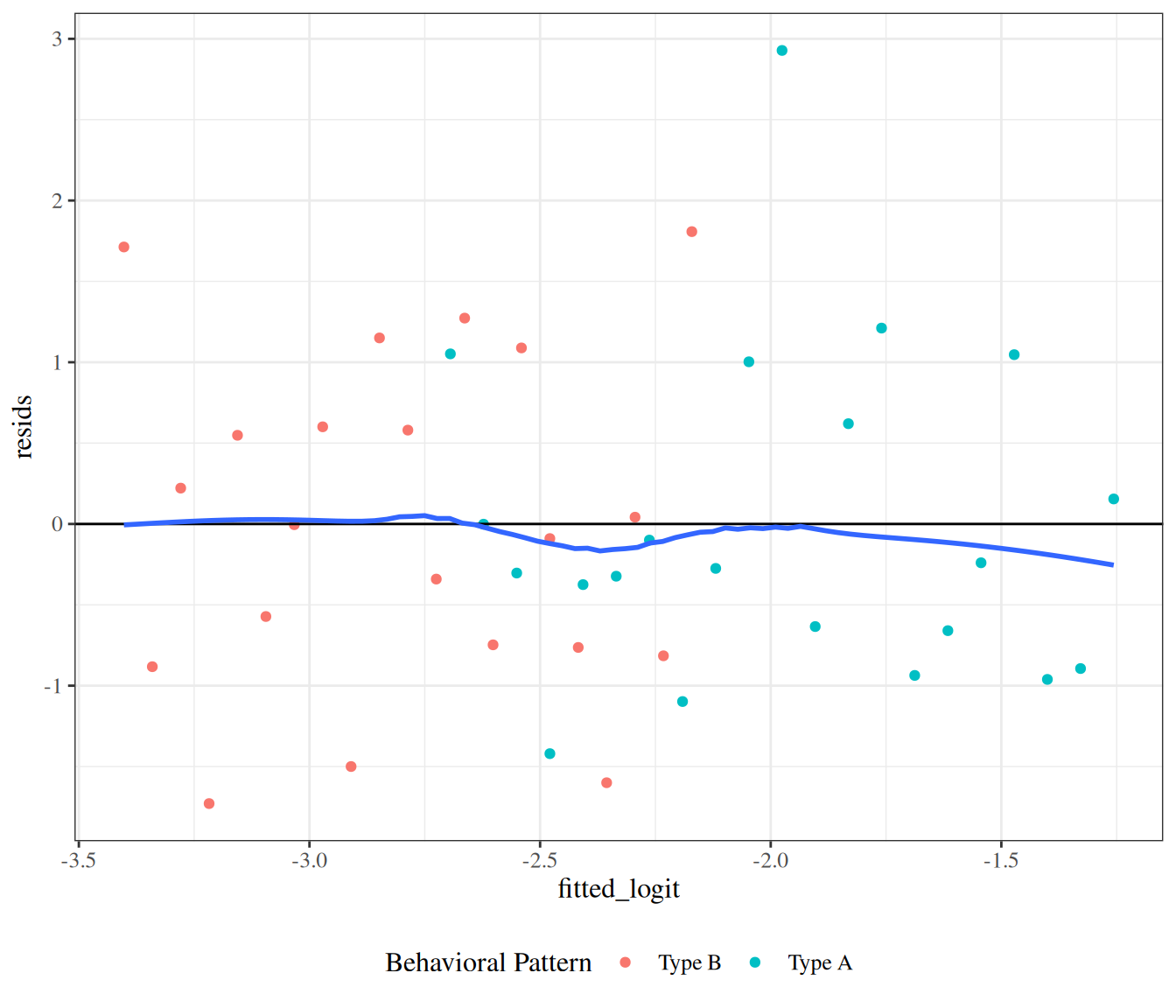
Example 10 (Pearson residuals for the WCGS CHD model) Let’s take a look at the Pearson residuals (Definition 8) for our CHD model from the WCGS data (graphed against the fitted values on the logit scale):

library(ggfortify)

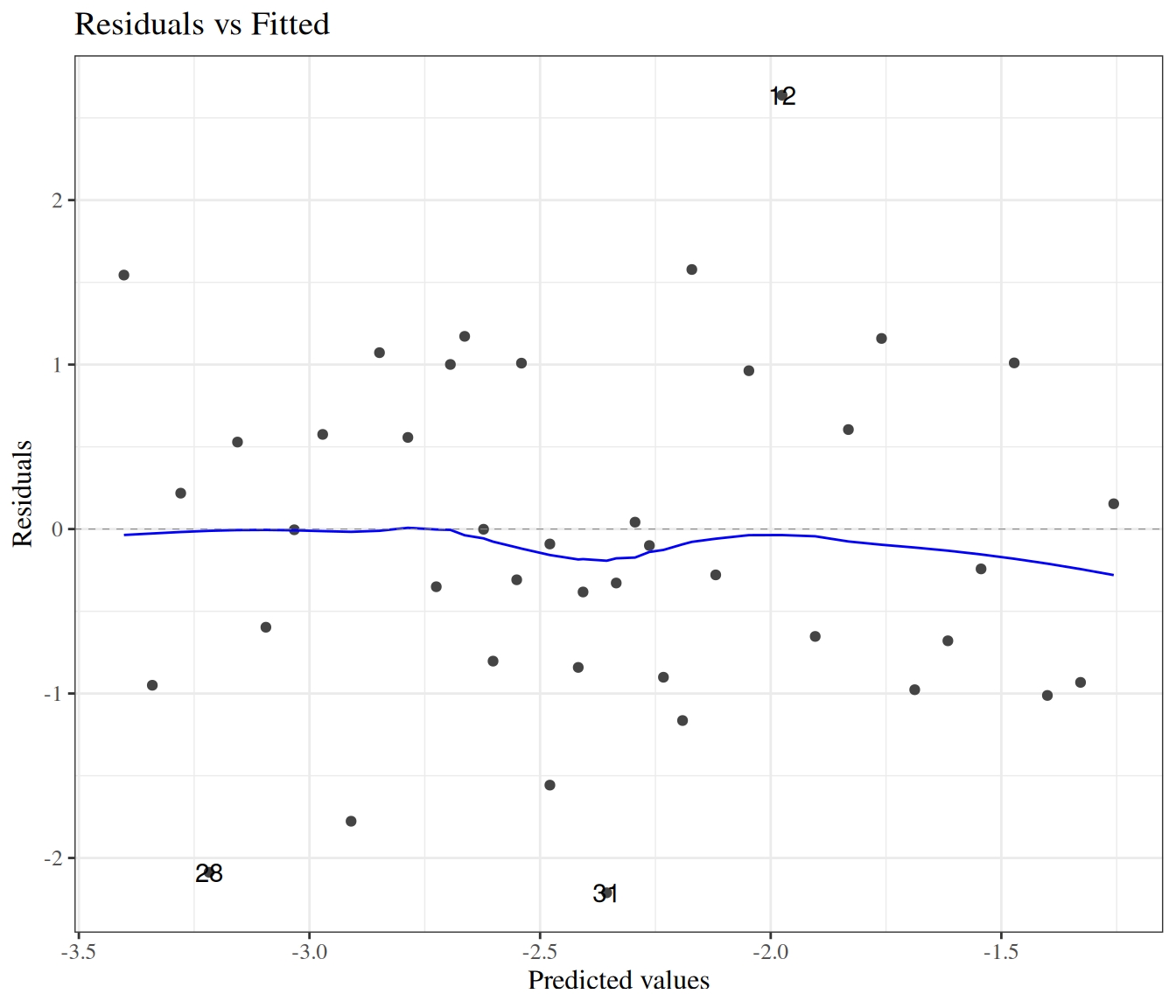
autoplot(chd_glm_contrasts_grouped, which = 1, ncol = 1) |> print()

The fan-shape is gone, and these residuals don’t show any obvious signs of model fit issues.

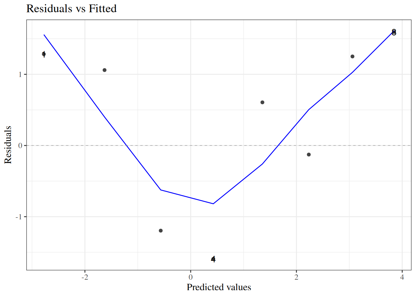
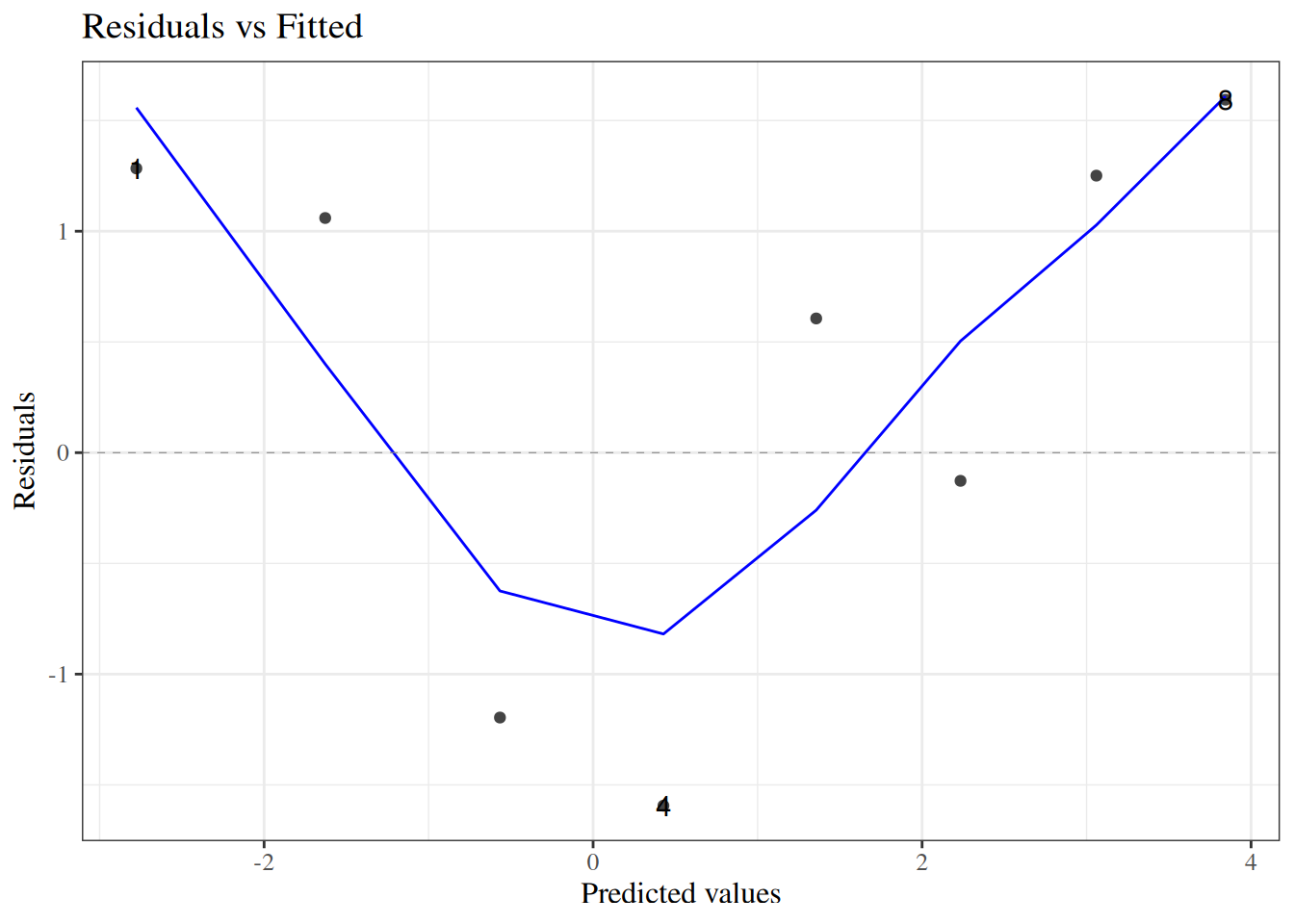
Example 11 (Counterexample: Pearson residuals for the beetles model) If we create the same plot for the beetles model, we see some strong evidence of a lack of fit; this plot is a counterexample to a well-fitting model:

library(glmx)
library(dplyr)
data(BeetleMortality)
beetles <- BeetleMortality |>
  mutate(
    pct = died / n,
    survived = n - died,
    dose_c = dose - mean(dose)
  )
beetles_glm_grouped <- beetles |>
  glm(
    formula = cbind(died, survived) ~ dose,
    family = "binomial"
  )
autoplot(beetles_glm_grouped, which = 1, ncol = 1) |> print()

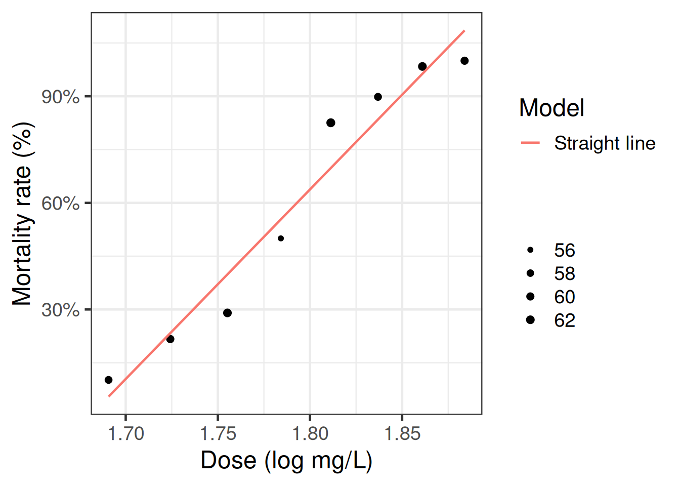
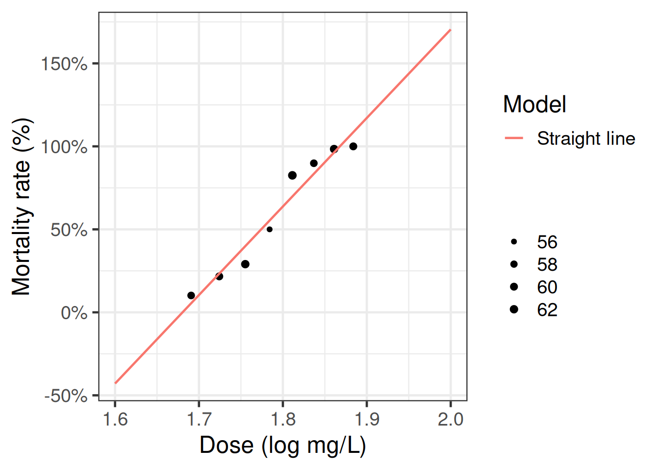
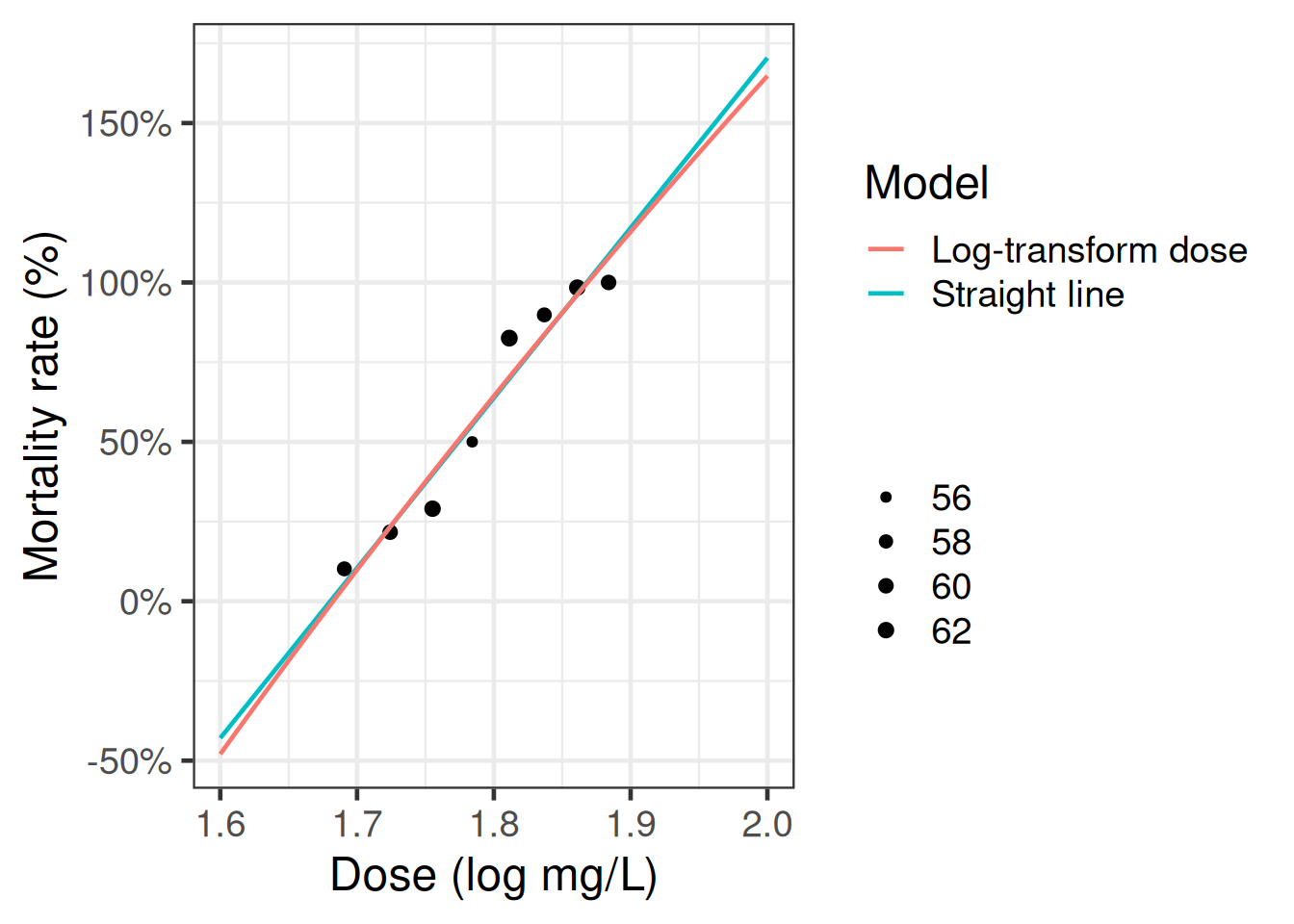
The clear pattern in the residuals signals that the straight-line logit model does not fit the beetle-mortality data well.

Pearson residuals with individual (ungrouped) data

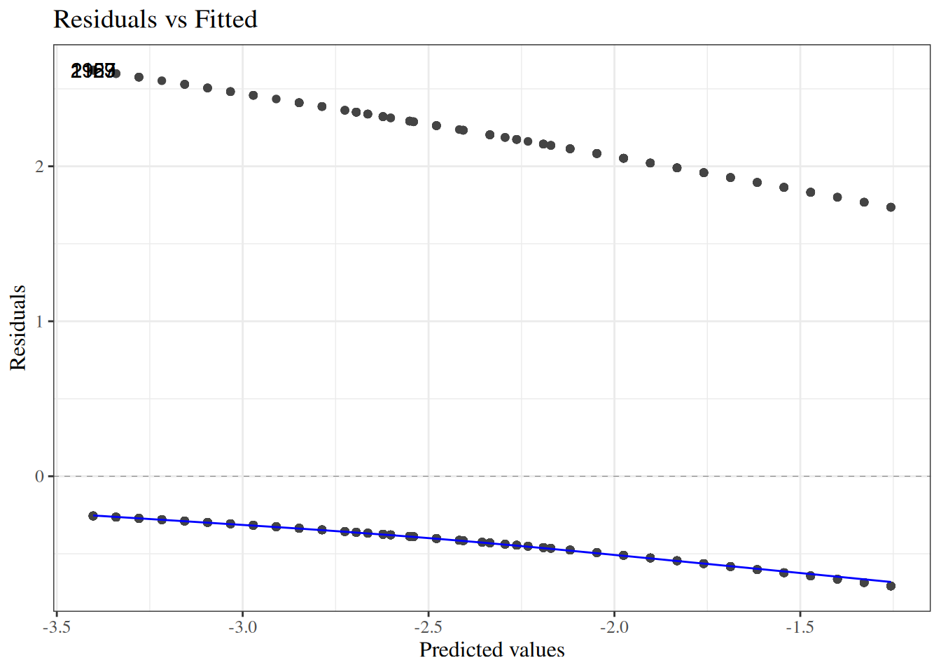
What happens if we try to compute residuals without grouping the data by covariate pattern?

library(ggfortify)

chd_glm_strat <- glm(
  "formula" = chd69 == "Yes" ~ dibpat + dibpat:age - 1,
  "data" = wcgs,
  "family" = binomial(link = "logit")
)

autoplot(chd_glm_strat, which = 1, ncol = 1) |> print()

This residuals-vs-fitted plot is meaningless: with ungrouped (individual-level) data, each covariate pattern contains only one observation (\(n_k = 1\)), so each residual can take only one of two possible values, both determined by the fitted probability \(\hat\pi(x_k)\) (one value when \(y_k = 1\) and another when \(y_k = 0\)). With a single binary observation per covariate pattern, the residuals have no meaningful reference distribution to assess the model fit against; this lack of a reference distribution is why logistic regression residuals only work for grouped data, with multiple observations per covariate pattern.

Residuals plot by hand

If you want to check your understanding of what these residual plots are, try building them yourself:

wcgs_grouped <-
  wcgs_grouped |>
  mutate(
    fitted = chd_glm_contrasts_grouped |> fitted(),
    fitted_logit = fitted |> logit(),
    resids = chd_glm_contrasts_grouped |> resid(type = "pearson")
  )

wcgs_resid_plot1 <-
  wcgs_grouped |>
  ggplot(
    mapping = aes(
      x = fitted_logit,
      y = resids
    )
  ) +
  geom_point(
    aes(col = dibpat)
  ) +
  geom_hline(yintercept = 0) +
  geom_smooth(
    se = FALSE,
    method.args = list(
      span = 2 / 3,
      degree = 1,
      family = "symmetric",
      iterations = 3,
      surface = "direct"
    ),
    method = stats::loess
  )
# plot.glm and autoplot use stats::lowess, which is hard to use with
# geom_smooth and hard to match exactly;
# see https://support.bioconductor.org/p/2323/

wcgs_resid_plot1 |> print()

Pearson chi-squared goodness of fit test

The Pearson chi-squared goodness of fit statistic is: \[X^2 = \sum_{k=1}^q X_k^2\]

Under the null hypothesis that the model in question is correct (i.e., sufficiently complex), \(X^2\ \dot \sim\ \chi^2(q-p)\).

x_pearson <- chd_glm_contrasts_grouped |>
  resid(type = "pearson")

chisq_stat <- sum(x_pearson^2)

pval <- pchisq(
  chisq_stat,
  lower = FALSE,
  df = length(x_pearson) - length(coef(chd_glm_contrasts_grouped))
)

For our CHD model, the p-value for this test is 0.265236; no significant evidence of a lack of fit at the 0.05 level.

Definition 9 (Leverage for a GLM) For a logistic (or other) generalized linear model fit to \(q\) covariate patterns with \(p\) parameters, the weighted hat matrix is

\[ \underbrace{\mathbf{H}}_{q \times q} \stackrel{\text{def}}{=} \underbrace{\mathbf{W}^{1/2}}_{q \times q} \underbrace{\mathbf{X}}_{q \times p} \mathopen{}\left(\underbrace{{\mathbf{X}}^{\top}\,\mathbf{W}\,\mathbf{X}}_{p \times p}\right)\mathclose{}^{-1} \underbrace{{\mathbf{X}}^{\top}}_{p \times q} \underbrace{\mathbf{W}^{1/2}}_{q \times q} \]

where \(\underbrace{\mathbf{W}}_{q \times q} \stackrel{\text{def}}{=}\text{diag}\mathopen{}\left(n_k \, \hat\pi_k \, (1 - \hat\pi_k)\right)\mathclose{}\) is the diagonal matrix of binomial weights, and the leverage \(h_k\) of covariate pattern \(k\) is the \(k\)-th diagonal element of \(\mathbf{H}\).

This weighted hat matrix is the GLM analog of the linear-model hat matrix; the weight matrix \(\mathbf{W}\) reduces to the identity in the ordinary-least-squares case.

Definition 10 (Standardized Pearson residual) Especially for small data sets, we might want to adjust our residuals for leverage (since outliers in \(X\) add extra variance to the residuals):

\[r_{P_k} \stackrel{\text{def}}{=}\frac{X_k}{\sqrt{1-h_k}}\]

where \(X_k\) is the Pearson residual (Definition 8) and \(h_k\) is the leverage of covariate pattern \(k\) (Definition 9). The functions autoplot() and plot.lm() use these for some of their graphs.

Deviance residuals

For large sample sizes, the Pearson and deviance residuals will be approximately the same. For small sample sizes, the deviance residuals from covariate patterns with small sample sizes can be unreliable (high variance).

Definition 11 (Deviance residual) Here \(\ell_{\text{full}}(x_k)\) is the saturated model’s log-likelihood contribution from covariate pattern \(k\), so that summing over the covariate patterns gives the full log-likelihood:

\[\ell_{\text{full}} \stackrel{\text{def}}{=}\sum_{k} \ell_{\text{full}}(x_k)\]

The deviance residual for covariate pattern \(k\) is

\[d_k \stackrel{\text{def}}{=}\operatorname{sign}(y_k - n_k \hat \pi_k)\left\{\sqrt{2[\ell_{\text{full}}(x_k) - \ell(\hat\beta; x_k)]}\right\}\]

Standardized deviance residuals

Analogously to the standardized Pearson residual (Definition 10), we can adjust the deviance residual for leverage:

\[r_{D_k} \stackrel{\text{def}}{=}\frac{d_k}{\sqrt{1-h_k}}\]

where \(h_k\) is the leverage of covariate pattern \(k\) (Definition 9).

Diagnostic plots

Definition 12  

Cook’s distance for a GLM

Some of the autoplot() diagnostic panels display Cook’s distance, which measures how influential each covariate pattern is on the fit. For a generalized linear model, the Cook’s distance for covariate pattern \(k\) combines the standardized Pearson residual (Definition 10) and the leverage (Definition 9):

\[D_k \stackrel{\text{def}}{=}\frac{(r_{P_k})^2}{p} \cdot \frac{h_k}{1 - h_k}\]

where \(p\) is the number of parameters. This diagnostic is the GLM analog of Cook’s distance for linear models, and shares its closed-form structure.

Example 12 (Diagnostics for the WCGS CHD model) Let’s take a look at the full set of autoplot() diagnostics now for our CHD model:

chd_glm_contrasts_grouped |>
  autoplot(which = 1:6) |>
  print()

Figure 20: Diagnostics for CHD model

Things look pretty good here. The QQ plot is still usable: when the number of observations at each covariate pattern is large, the grouped residuals should be approximately Gaussian.

Example 13 (Diagnostics for the beetles model) Let’s look at the beetles model diagnostic plots for comparison:

beetles_glm_grouped |>
  autoplot(which = 1:6) |>
  print()

Figure 21: Diagnostics for logistic model of BeetleMortality data

Hard to tell much from so little data, but there might be some issues here.

10 Alternatives to reporting odds ratios

10.1 Objections to odds ratios

Some scholars have raised objections to the use of odds ratios as an effect measurement (Sackett et al. 1996; Norton et al. 2024).

As we saw in the figure comparing risk differences, risk ratios, and odds ratios, the odds ratio is not very closely correlated with the risk difference, and the risk difference is typically the metric that ultimately matters for policy decisions.

Another objection is that odds ratios (and risk ratios, and risk differences) depend on the set of covariates in a logistic regression model, even when those covariates are independent of the exposure of interest and do not interact with that exposure. For example, consider the following model:

\[\operatorname{P}(Y=y|X=x,C=c) = {\color{red}{\pi(x,c)}}^y (1-{\color{red}{\pi(x,c)}})^{1-y}\]

\[{\color{red}{\pi(x,c)}} = \operatorname{expit}\mathopen{}\left\{\eta_0 + \beta_Xx + \beta_Cc\right\}\mathclose{} \tag{39}\]

Then:

\[ \begin{aligned} \operatorname{E}\mathopen{}\left[Y|X=x\right]\mathclose{} &= \operatorname{E}\mathopen{}\left[\operatorname{E}\mathopen{}\left[Y | X, C\right]\mathclose{} | X=x\right]\mathclose{} && \text{(law of total expectation)} \\ &= \operatorname{E}\mathopen{}\left[{\color{red}{\pi(X,C)}} | X=x\right]\mathclose{} && \text{(Bernoulli conditional mean: } \operatorname{E}\mathopen{}\left[Y|X,C\right]\mathclose{} = \pi(X,C) \text{)} \\ &= \operatorname{E}\mathopen{}\left[\operatorname{expit}\mathopen{}\left\{\eta_0 + \beta_X X + \beta_C C\right\}\mathclose{} | X=x\right]\mathclose{} && \text{(model definition of } \pi \text{)} \\ &= \operatorname{E}\mathopen{}\left[\operatorname{expit}\mathopen{}\left\{\eta_0 + \beta_X x + \beta_C C\right\}\mathclose{} | X=x\right]\mathclose{} && \text{(conditioning on } X = x \text{ fixes } X \text{ at } x \text{)} \\ &= \int_c{\operatorname{expit}\mathopen{}\left\{\eta_0 + \beta_X x + \beta_C c\right\}\mathclose{} ~\operatorname{p}(C=c|X=x)~ \partial c} && \text{(conditional expectation as an integral over } C \text{'s conditional distribution)} \\ &= \int_c{{\color{red}{\pi(x,c)}}~ \operatorname{p}(C=c|X=x)~ \partial c} && \text{(model definition of } \pi \text{, in reverse)} \end{aligned} \]

Since the \(\operatorname{expit}\mathopen{}\left\{\right\}\mathclose{}\) function is nonlinear, we can’t change the order of the expectation and \(\operatorname{expit}\mathopen{}\left\{\right\}\mathclose{}\) operators:

\[\operatorname{E}\mathopen{}\left[\operatorname{expit}\mathopen{}\left\{\eta_0 + \beta_XX + \beta_CC\right\}\mathclose{} | X\right]\mathclose{} \neq \operatorname{expit}\mathopen{}\left\{\operatorname{E}\mathopen{}\left[\eta_0 + \beta_XX + \beta_CC\right]\mathclose{} | X\right\}\mathclose{}\]

In contrast, consider a model with an identity link function:

\[\operatorname{P}(Y=y|X=x,C=c) = {\color{red}{\pi(x,c)}}^y (1-{\color{red}{\pi(x,c)}})^{1-y}\]

\[{\color{red}{\pi(x,c)}} = \eta_0 + \beta_Xx + \beta_Cc \tag{40}\]

Then:

\[ \begin{aligned} \operatorname{E}\mathopen{}\left[Y|X=x\right]\mathclose{} &= \operatorname{E}\mathopen{}\left[\operatorname{E}\mathopen{}\left[Y | X, C\right]\mathclose{} | X=x\right]\mathclose{} && \text{(law of total expectation)} \\ &= \operatorname{E}\mathopen{}\left[{\color{red}{\pi(X,C)}} | X=x\right]\mathclose{} && \text{(Bernoulli conditional mean: } \operatorname{E}\mathopen{}\left[Y|X,C\right]\mathclose{} = \pi(X,C) \text{)} \\ &= \operatorname{E}\mathopen{}\left[\eta_0 + \beta_X X + \beta_C C | X=x\right]\mathclose{} && \text{(identity-link model definition of } \pi \text{)} \\ &= \operatorname{E}\mathopen{}\left[\eta_0 | X=x\right]\mathclose{} + \operatorname{E}\mathopen{}\left[\beta_X X | X=x\right]\mathclose{} + \operatorname{E}\mathopen{}\left[\beta_C C | X=x\right]\mathclose{} && \text{(linearity of expectation)} \\ &= \eta_0 + \operatorname{E}\mathopen{}\left[\beta_X X | X=x\right]\mathclose{} + \operatorname{E}\mathopen{}\left[\beta_C C | X=x\right]\mathclose{} && \text{(expectation of a constant)} \\ &= \eta_0 + \beta_X \operatorname{E}\mathopen{}\left[X | X=x\right]\mathclose{} + \beta_C \operatorname{E}\mathopen{}\left[C | X=x\right]\mathclose{} && \text{(constant factors move outside expectations)} \\ &= \eta_0 + \beta_X x + \beta_C \operatorname{E}\mathopen{}\left[C | X=x\right]\mathclose{} && \text{(} \operatorname{E}\mathopen{}\left[X | X=x\right]\mathclose{} = x \text{)} \\ &= {\color{red}{(\eta_0 + \beta_C\operatorname{E}\mathopen{}\left[C | X=x\right]\mathclose{})}} + {\color{teal}{\beta_Xx}} && \text{(commute and regroup the terms)} \end{aligned} \]

If \(C \perp\!\!\!\perp X\), then \(\operatorname{E}\mathopen{}\left[C|X=x\right]\mathclose{} = \operatorname{E}\mathopen{}\left[C\right]\mathclose{}\), and we can simplify further:

\[ \begin{aligned} \operatorname{E}\mathopen{}\left[Y|X=x\right]\mathclose{} &= {\color{red}{(\eta_0 + \beta_C \operatorname{E}\mathopen{}\left[C|X=x\right]\mathclose{})}} + {\color{teal}{\beta_Xx}} && \text{(marginal mean under the identity link)} \\ &= {\color{red}{(\eta_0 + \beta_C \operatorname{E}\mathopen{}\left[C\right]\mathclose{})}} + {\color{teal}{\beta_Xx}} && \text{(} C \perp\!\!\!\perp X \text{, so } \operatorname{E}\mathopen{}\left[C|X=x\right]\mathclose{} = \operatorname{E}\mathopen{}\left[C\right]\mathclose{} \text{)} \\&= {\color{red}{\eta_0^*}} + {\color{teal}{\beta_Xx}} && \text{(definition: } \eta_0^* \stackrel{\text{def}}{=}\eta_0 + \beta_C \operatorname{E}\mathopen{}\left[C\right]\mathclose{} \text{)} \end{aligned} \]

Then:

\[ \begin{aligned} \frac{\partial}{\partial x} \operatorname{E}\mathopen{}\left[Y|X=x\right]\mathclose{} &= \frac{\partial}{\partial x} \mathopen{}\left({\color{red}{\eta_0^*}} + {\color{teal}{\beta_Xx}}\right)\mathclose{} && \text{(marginal mean when } C \perp\!\!\!\perp X \text{)} \\ &= \frac{\partial}{\partial x}\eta_0^* + \frac{\partial}{\partial x}\mathopen{}\left(\beta_X x\right)\mathclose{} && \text{(linearity of differentiation)} \\ &= 0 + \frac{\partial}{\partial x}\mathopen{}\left(\beta_X x\right)\mathclose{} && \text{(} \eta_0^* \text{ does not depend on } x \text{)} \\ &= 0 + \beta_X && \text{(derivative of a linear term)} \\ &= {\color{teal}{\beta_X}} && \text{(additive identity)} \end{aligned} \]

The conditional slope is the same:

\[ \begin{aligned} \frac{\partial}{\partial x} \operatorname{E}\mathopen{}\left[Y|X=x,C=c\right]\mathclose{} &= \frac{\partial}{\partial x} \mathopen{}\left(\eta_0 + \beta_Xx + \beta_Cc\right)\mathclose{} && \text{(identity-link model definition of } \pi \text{)} \\ &= 0 + \beta_X + 0 && \text{(term-by-term: only } \beta_X x \text{ depends on } x \text{)} \\ &= {\color{teal}{\beta_X}} && \text{(additive identity)} \end{aligned} \]

Therefore:

\[ \frac{\partial}{\partial x} \operatorname{E}\mathopen{}\left[Y|X=x\right]\mathclose{} = {\color{teal}{\beta_X}} = \frac{\partial}{\partial x} \operatorname{E}\mathopen{}\left[Y|X=x,C=c\right]\mathclose{} \]

In other words, for a model with an identity link function, if covariates \(X\) and \(C\) are independent, then the slope with respect to \(X\) doesn’t depend on whether \(C\) is included in the model (and an analogous result holds if \(X\) is discrete or categorical).

Exercise 27 What are the expressions for \(\operatorname{E}\mathopen{}\left[Y|X=x\right]\mathclose{}\) and \(\frac{\partial}{\partial x} \operatorname{E}\mathopen{}\left[Y|X=x\right]\mathclose{}\) for the identity-link model in Equation 40, if \(\operatorname{E}\mathopen{}\left[C|X=x\right]\mathclose{} = \gamma_0 + \gamma_x x\)?

Solution 27. \[ \begin{aligned} \operatorname{E}\mathopen{}\left[Y|X=x\right]\mathclose{} &= \operatorname{E}\mathopen{}\left[\pi(x, C)|X=x\right]\mathclose{} && \text{(law of total expectation, conditional on } X = x \text{)} \\ &= \operatorname{E}\mathopen{}\left[\eta_0 + \beta_Xx + \beta_C C|X=x\right]\mathclose{} && \text{(identity-link model)} \\ &= \eta_0 + \beta_Xx + \beta_C \operatorname{E}\mathopen{}\left[C|X=x\right]\mathclose{} && \text{(linearity of expectation)} \\ &= \eta_0 + \beta_Xx + \beta_C (\gamma_0 + \gamma_x x) && \text{(substitute } \operatorname{E}\mathopen{}\left[C|X=x\right]\mathclose{} = \gamma_0 + \gamma_x x \text{)} \\ &= \eta_0 + \beta_Xx + \beta_C \gamma_0 + \beta_C \gamma_x x && \text{(distribute)} \\ &= (\eta_0 + \beta_C \gamma_0) + (\beta_X + \beta_C \gamma_x) x && \text{(commute and regroup the terms)} \end{aligned} \]

\[ \begin{aligned} \frac{\partial}{\partial x}\operatorname{E}\mathopen{}\left[Y|X=x\right]\mathclose{} &= \frac{\partial}{\partial x}\mathopen{}\left\{(\eta_0 + \beta_C \gamma_0) + (\beta_X + \beta_C \gamma_x) x\right\}\mathclose{} && \text{(marginal mean from the derivation of } \operatorname{E}\mathopen{}\left[Y|X=x\right]\mathclose{} \text{)} \\ &= \frac{\partial}{\partial x}(\eta_0 + \beta_C \gamma_0) + \frac{\partial}{\partial x}\mathopen{}\left\{(\beta_X + \beta_C \gamma_x) x\right\}\mathclose{} && \text{(linearity of differentiation)} \\ &= \beta_X + \beta_C \gamma_x && \text{(constants have derivative 0; derivative of a linear term)} \end{aligned} \]

The marginal mean is still linear in \(x\), but its slope \(\beta_X + \beta_C \gamma_x\) differs from the conditional slope \(\beta_X\) unless \(\beta_C = 0\) or \(\gamma_x = 0\).

Exercise 28 What are the expressions for \(\operatorname{E}\mathopen{}\left[Y|X=x\right]\mathclose{}\) and \(\frac{\partial}{\partial x} \operatorname{E}\mathopen{}\left[Y|X=x\right]\mathclose{}\), if instead of the identity-link model in Equation 40, \[\pi(x,c) = \eta_0 + \beta_Xx + \beta_Cc +\beta_{XC}xc\] and \(\operatorname{E}\mathopen{}\left[C|X=x\right]\mathclose{} = \gamma_0 + \gamma_x x\)?

Solution 28. \[ \begin{aligned} \operatorname{E}\mathopen{}\left[Y|X=x\right]\mathclose{} &= \operatorname{E}\mathopen{}\left[\pi(x, C)|X=x\right]\mathclose{} && \text{(law of total expectation, conditional on } X = x \text{)} \\ &= \operatorname{E}\mathopen{}\left[\eta_0 + \beta_Xx + \beta_C C + \beta_{XC}xC|X=x\right]\mathclose{} && \text{(interaction model)} \\ &= \eta_0 + \beta_Xx + \beta_C \operatorname{E}\mathopen{}\left[C|X=x\right]\mathclose{} + \beta_{XC}x \operatorname{E}\mathopen{}\left[C|X=x\right]\mathclose{} && \text{(linearity of expectation)} \\ &= \eta_0 + \beta_Xx + (\beta_C + \beta_{XC}x)\operatorname{E}\mathopen{}\left[C|X=x\right]\mathclose{} && \text{(factor out } \operatorname{E}\mathopen{}\left[C|X=x\right]\mathclose{} \text{)} \\ &= \eta_0 + \beta_Xx + (\beta_C + \beta_{XC}x)(\gamma_0 + \gamma_x x) && \text{(substitute } \operatorname{E}\mathopen{}\left[C|X=x\right]\mathclose{} = \gamma_0 + \gamma_x x \text{)} \\ &= \eta_0 + \beta_Xx + \beta_C\gamma_0 + \beta_C\gamma_x x + \beta_{XC}\gamma_0 x + \beta_{XC}\gamma_x x^2 && \text{(distribute)} \\ &= (\eta_0 + \beta_C\gamma_0) + (\beta_X + \beta_C\gamma_x + \beta_{XC}\gamma_0) x + \beta_{XC}\gamma_x x^2 && \text{(commute and regroup the terms)} \end{aligned} \]

\[ \begin{aligned} \frac{\partial}{\partial x}\operatorname{E}\mathopen{}\left[Y|X=x\right]\mathclose{} &= \frac{\partial}{\partial x}\mathopen{}\left\{(\eta_0 + \beta_C\gamma_0) + (\beta_X + \beta_C\gamma_x + \beta_{XC}\gamma_0) x + \beta_{XC}\gamma_x x^2\right\}\mathclose{} && \text{(marginal mean from the derivation of } \operatorname{E}\mathopen{}\left[Y|X=x\right]\mathclose{} \text{)} \\ &= \frac{\partial}{\partial x}(\eta_0 + \beta_C\gamma_0) + \frac{\partial}{\partial x}\mathopen{}\left\{(\beta_X + \beta_C\gamma_x + \beta_{XC}\gamma_0) x\right\}\mathclose{} + \frac{\partial}{\partial x}\mathopen{}\left(\beta_{XC}\gamma_x x^2\right)\mathclose{} && \text{(linearity of differentiation)} \\ &= (\beta_X + \beta_C\gamma_x + \beta_{XC}\gamma_0) + 2\beta_{XC}\gamma_x x && \text{(constants have derivative 0; derivative of a linear term; power rule)} \end{aligned} \]

So, answering the hint: yes — adding the interaction term changes the functional form of \(\operatorname{E}\mathopen{}\left[Y|X=x\right]\mathclose{}\). The marginal mean is now quadratic in \(x\) (whenever \(\beta_{XC} \neq 0\) and \(\gamma_x \neq 0\)), even though the conditional model is linear in \(x\) for each fixed \(c\), and the marginal slope now varies with \(x\).

10.2 Deriving risk ratios and risk differences from logistic regression models

If you want to report risk differences or risk ratios instead of odds ratios, you can obtain estimates from logistic regression models, as long as you didn’t stratify sampling by the outcome; in other words, not in case-control studies (see Odds Ratios in Case-Control Studies).

Computing marginal risk differences

Note

This section is optional for 2026 and will not be tested on exams.

Conceptual approach

To compute risk ratios or risk differences from logistic regression models:

• Apply the expit function (definition) to the linear predictor for each covariate pattern to compute the (estimated) risks,
• Then take the differences or ratios of the risks, as needed.

For example, suppose we have a logistic regression model with a binary exposure \(A\) and a covariate \(Z\):

\[ \operatorname{logit}\mathopen{}\left\{\Pr(Y = 1 | A, Z)\right\}\mathclose{} = \beta_0 + \beta_A A + \beta_Z Z \tag{41}\]

Definition 13 (Conditional predicted risk) The conditional predicted risk (or conditional risk) for an individual with exposure \(A = a\) and covariate \(Z = z\) is the population probability

\[ \pi(a, z) \stackrel{\text{def}}{=}\Pr(Y = 1 \mid A = a, Z = z). \]

Under the logistic model in Equation 41, this population risk equals

\[ \pi(a, z) = \operatorname{expit}\mathopen{}\left\{\beta_0 + \beta_A a + \beta_Z z\right\}\mathclose{}. \]

Definition 14 (Conditional risk difference) The conditional risk difference comparing exposure levels \(a = 1\) vs. \(a = 0\) at a fixed covariate value \(z\) is, using the conditional predicted risk (Definition 13):

\[ \text{RD}(z) \stackrel{\text{def}}{=}\pi(1, z) - \pi(0, z) \]

Definition 15 (Conditional risk ratio) The conditional risk ratio comparing exposure levels \(a = 1\) vs. \(a = 0\) at a fixed covariate value \(z\) is, using the conditional predicted risk (Definition 13):

\[ \text{RR}(z) \stackrel{\text{def}}{=}\frac{\pi(1, z)}{\pi(0, z)} \]

Example 14 (Numerical example: conditional RD and RR at a fixed covariate value) Using the WCGS data with dibpat (behavior pattern) as the exposure and chd69 (coronary heart disease by 1969) as the outcome, adjusted for age:

library(dplyr)
library(haven)

wcgs_clean <- rmb::wcgs |>
  mutate(
    across(where(is.labelled), haven::as_factor),
    dibpat = dibpat |> relevel(ref = "Type B"),
    chd69_binary = as.numeric(chd69 == "Yes")
  ) |>
  filter(!is.na(chd69_binary), !is.na(dibpat), !is.na(age))

fit <- glm(
  chd69_binary ~ dibpat + age,
  data = wcgs_clean,
  family = binomial(link = "logit")
)

At age \(z = 50\) (within the WCGS sample’s observed age range):

z <- 50
dibpat_levels <- levels(wcgs_clean$dibpat)
wcgs_cf_a <- data.frame(dibpat = factor("Type A", levels = dibpat_levels), age = z)
wcgs_cf_b <- data.frame(dibpat = factor("Type B", levels = dibpat_levels), age = z)

pi_hat_1 <- predict(fit, newdata = wcgs_cf_a, type = "response")
pi_hat_0 <- predict(fit, newdata = wcgs_cf_b, type = "response")

rd_hat_z <- pi_hat_1 - pi_hat_0
rr_hat_z <- pi_hat_1 / pi_hat_0

tibble::tibble(
  quantity = c(
    "$\\hat\\pi(1, 50)$", "$\\hat\\pi(0, 50)$",
    "$\\widehat{\\text{RD}}(50)$", "$\\widehat{\\text{RR}}(50)$"
  ),
  value = c(pi_hat_1, pi_hat_0, rd_hat_z, rr_hat_z)
) |>
  knitr::kable(digits = 3)

quantity	value
\(\hat\pi(1, 50)\)	0.129
\(\hat\pi(0, 50)\)	0.063
\(\widehat{\text{RD}}(50)\)	0.067
\(\widehat{\text{RR}}(50)\)	2.066

These are conditional estimates: both hold age fixed at 50 and compare only the two exposure levels at that one age.

Marginal vs. conditional effects

Note that these risk differences and risk ratios are conditional on the covariate value \(z\). In many applications, we want to summarize the effect across the population, which requires computing a marginal risk difference or risk ratio.

Definition 16 (Observed marginal risk) The observed marginal risk under exposure level \(A = a\) is:

\[\pi(a) \stackrel{\text{def}}{=}\Pr(Y = 1 \mid A = a)\]

Example 15 (Illustration: observed marginal risk) Continuing the WCGS example (Example 14):

pi1_direct <- mean(wcgs_clean$chd69_binary[wcgs_clean$dibpat == "Type A"])

The observed marginal risk among the Type A men (\(A = 1\)) is simply the proportion of them who developed CHD by 1969:

\[ \pi(1) = \Pr(Y = 1 \mid A = 1) = 0.112 \]

This definition collapses the outcome over everything else in one step. When the model also conditions on covariates \(Z\), we can unpack \(\pi(a)\) as the covariate-specific risk \(\pi(a, z)\) averaged over the distribution of \(Z\) among those with \(A = a\):

Theorem 14 (Marginal risk as a conditional expectation) \[\pi(a) = \operatorname{E}\mathopen{}\left[{\color{teal}{\pi(a, Z)}} \mid {\color{red}{A = a}}\right]\mathclose{}\]

where \({\color{teal}{\pi(a, z)}}\) is the conditional predicted risk (Definition 13).

Proof. \[ \begin{aligned} \pi(a) &= \Pr(Y = 1 \mid A = a) && \text{[definition of observed marginal risk]} \\ &= \int \Pr(Y = 1 \mid Z=z, A = a)\, {\color{red}{f_{Z \mid A}(z \mid a)}}\, dz && \text{[law of total probability]} \\ &= \int {\color{teal}{\pi(a, z)}}\, {\color{red}{f_{Z \mid A}(z \mid a)}}\, dz && \text{[definition of conditional risk]} \\ &= \operatorname{E}\mathopen{}\left[{\color{teal}{\pi(a, Z)}} \mid {\color{red}{A = a}}\right]\mathclose{} && \text{[definition of conditional expectation]} \end{aligned} \]

Example 16 (Observed marginal risk by standardization) Take \(Z\) to be an indicator for age 50 or older. Among the WCGS men with \(A = 1\) (Type A):

wcgs_clean$age_ge50 <- as.numeric(wcgs_clean$age >= 50)
wcgs_exposed <- wcgs_clean[wcgs_clean$dibpat == "Type A", ]
pi1_z0 <- mean(wcgs_exposed$chd69_binary[wcgs_exposed$age_ge50 == 0])
pi1_z1 <- mean(wcgs_exposed$chd69_binary[wcgs_exposed$age_ge50 == 1])
p_z1_a1 <- mean(wcgs_exposed$age_ge50)

the age-specific risks are \(\pi(1, 0) = 0.089\) (under 50) and \(\pi(1, 1) = 0.159\) (50 or older), and \(\Pr(Z = 1 \mid A = 1) = 0.329\) of the Type A men are 50 or older. Then Theorem 14 gives:

\[ \begin{aligned} \pi(1) &= \operatorname{E}\mathopen{}\left[\pi(1, Z) \mid A = 1\right]\mathclose{} && \text{[observed marginal risk theorem]} \\ &= (1 - 0.329)(0.089) + (0.329)(0.159) && \text{[substitute stratum risks and weights]} \\ &= 0.112 && \text{[arithmetic]} \end{aligned} \]

matching the direct estimate \(\pi(1) = 0.112\) from Example 15 (up to rounding).

Note

The rest of this section previews causal-inference concepts — potential outcomes, consistency, exchangeability, and positivity — that are formally defined and developed fully in the causal inference chapter.

In causal inference, potential outcomes \(Y^a\) represent the outcome each unit would have under exposure level \(a\). Population-level causal estimands summarize these potential outcomes:

Definition 17 (Potential mean) The potential mean (or mean potential outcome) under treatment \(A = a\) is the expected value of the potential outcome \(Y^a\):

\[\mu_a \stackrel{\text{def}}{=}\operatorname{E}\mathopen{}\left[Y^a\right]\mathclose{}\]

The potential mean is what the average outcome would be if the entire population were assigned treatment \(a\).

Example 17 (Illustration: potential mean) Suppose, hypothetically, that if every man in the WCGS cohort had exhibited Type A behavior pattern (\(a = 1\)), the fraction who would go on to develop CHD by 1969 were close to the fraction actually observed among the men who really did have that behavior pattern, \(\pi(1) = 0.112\) (Example 15). Under that supposition, the potential mean is \(\mu_1 = \operatorname{E}\mathopen{}\left[Y^1\right]\mathclose{} = 0.112\).

For a binary outcome, the potential mean is a probability, which we give its own name:

Definition 18 (Causal marginal risk) For a binary outcome \(Y \in \{0, 1\}\), the potential mean (Definition 17) is a probability, which we call the causal marginal risk (also: potential probability, potential marginal risk) under exposure level \(a\):

\[\pi_a \stackrel{\text{def}}{=}\Pr(Y^a = 1)\]

We use the term causal marginal risk throughout.

Example 18 (Illustration: causal marginal risk) Continuing Example 17, under that same supposition the causal marginal risk is \(\pi_1 = \Pr(Y^1 = 1) = 0.112\) — the fraction who would develop CHD if every man in the cohort had Type A behavior pattern.

Theorem 15 (Causal marginal risk equals potential mean) The matching values in Example 17 and Example 18 are no coincidence: the causal marginal risk (Definition 18) is a special case of the potential mean (Definition 17):

\[\pi_a = \operatorname{E}\mathopen{}\left[Y^a\right]\mathclose{}\]

Proof. Since \(Y^a\) is binary (\(Y^a \in \{0, 1\}\)):

\[ \begin{aligned} \operatorname{E}\mathopen{}\left[Y^a\right]\mathclose{} &= 1 \cdot \Pr(Y^a = 1) + 0 \cdot \Pr(Y^a = 0) && \text{[expectation of a binary variable]} \\ &= \Pr(Y^a = 1) && \text{[arithmetic]} \\ &= \pi_a && \text{[definition of causal marginal risk]} \end{aligned} \]

Example 19 (Illustration: causal marginal risk equals potential mean) With \(\pi_1 = 0.112\) as in Example 18, reading the potential mean as an expectation gives the same value:

\[ \operatorname{E}\mathopen{}\left[Y^1\right]\mathclose{} = 1 \cdot 0.112 + 0 \cdot 0.888 = 0.112 = \pi_1. \]

Under causal identification assumptions (see Consistency, Conditional Exchangeability, and Positivity), the causal marginal risk \(\pi_a\) (Definition 18) can be expressed in terms of observed data:

Theorem 16 (Causal marginal risk under identification assumptions) Under Consistency, Conditional Exchangeability, and Positivity:

\[\pi_a = \operatorname{E}\mathopen{}\left[{\color{teal}{\pi(a, Z)}}\right]\mathclose{}\]

where the expectation is over the marginal distribution of \(Z\) (not the conditional distribution \(f_{Z \mid A}(z \mid a)\)).

Proof. \[ \begin{aligned} \pi_a &= \Pr(Y^a = 1) && \text{[definition of causal marginal risk]} \\ &= \int \Pr(Y^a = 1 \mid Z=z)\, {\color{red}{f_Z(z)}}\, dz && \text{[law of total probability]} \\ &= \int \Pr(Y^a = 1 \mid A=a, Z=z)\, {\color{red}{f_Z(z)}}\, dz && \text{[by conditional exchangeability]} \\ &= \int \Pr(Y=1 \mid A=a, Z=z)\, {\color{red}{f_Z(z)}}\, dz && \text{[by consistency]} \\ &= \int {\color{teal}{\pi(a, z)}}\, {\color{red}{f_Z(z)}}\, dz && \text{[definition of conditional risk]} \\ &= \operatorname{E}\mathopen{}\left[{\color{teal}{\pi(a, Z)}}\right]\mathclose{} && \text{[definition of expectation]} \end{aligned} \]

Conditional exchangeability licenses adding the conditioning on \(A = a\); positivity (\(\Pr(A = a \mid Z = z) > 0\) wherever \(f_Z(z) > 0\)) guarantees that conditional risk is defined in every stratum; and consistency replaces the potential outcome \(Y^a\) with the observed \(Y\).

Example 20 (Causal marginal risk by standardization) Continuing Example 16 with the same age-specific risks \(\pi(1, 0) = 0.089\) and \(\pi(1, 1) = 0.159\), now weight by the age distribution of the whole WCGS population rather than just the Type A men:

p_z1_pop <- mean(wcgs_clean$age_ge50)

\(\Pr(Z = 1) = 0.287\) of the whole population is 50 or older — a smaller share than among the Type A men (\(\Pr(Z = 1 \mid A = 1) = 0.329\)), since behavior pattern and age are associated in this cohort. Then Theorem 16 gives:

\[ \begin{aligned} \pi_1 &= \operatorname{E}\mathopen{}\left[\pi(1, Z)\right]\mathclose{} && \text{[causal marginal risk theorem]} \\ &= (1 - 0.287)(0.089) + (0.287)(0.159) && \text{[substitute stratum risks and weights]} \\ &= 0.109 && \text{[arithmetic]} \end{aligned} \]

This causal marginal risk differs (slightly) from the observed marginal risk \(\pi(1) = 0.112\) because the Type A men skew somewhat older than the WCGS population as a whole.

We can now place the observed and causal marginal risks side by side:

Remark 2 (Observed vs. causal marginal risk). The two risks differ in what they define — one conditions on the observed exposure \(A = a\), the other on a potential outcome \(Y^a\) — and, once unpacked through \({\color{teal}{\pi(a, z)}} = \Pr(Y = 1 \mid A = a, Z = z)\), in the distribution of \(Z\) they average over:

\[ \begin{aligned} \text{observed: } \quad \pi(a) &= \Pr(Y=1 \mid {\color{red}{A=a}}) &&= \operatorname{E}\mathopen{}\left[{\color{teal}{\pi(a, Z)}} \mid {\color{red}{A = a}}\right]\mathclose{} &&= \int {\color{teal}{\pi(a, z)}}\, {\color{red}{f_{Z \mid A}(z \mid a)}}\, dz \\ \text{causal: } \quad \pi_a &= \Pr({\color{red}{Y^a}}=1) &&= \operatorname{E}\mathopen{}\left[{\color{teal}{\pi(a, Z)}}\right]\mathclose{} &&= \int {\color{teal}{\pi(a, z)}}\, {\color{red}{f_{Z}(z)}}\, dz \end{aligned} \]

The observed marginal risk \(\pi(a)\) (Theorem 14) weights \({\color{teal}{\pi(a, z)}}\) by the covariate distribution \({\color{red}{f_{Z \mid A}(z \mid a)}}\) among those actually exposed to \(A = a\), so it inherits any association between \(A\) and \(Z\) (that is, any confounding).

The causal marginal risk \(\pi_a\) (Theorem 16) weights \({\color{teal}{\pi(a, z)}}\) by the whole population’s covariate distribution \({\color{red}{f_{Z}(z)}}\), which is the same for every exposure level \(a\); that common weighting is what makes the causal contrast \(\pi_1 - \pi_0\) an apples-to-apples comparison.

When \(A\) and \(Z\) are associated, the two risks diverge; they coincide in the absence of such association.

Corollary 9 (Observed and causal marginal risks coincide without confounding) Assume Consistency, Conditional Exchangeability, Positivity, and \(Z \perp\!\!\!\perp A\). Then the observed and causal marginal risks are equal:

\[\pi(a) = \pi_a\]

Proof. When \(Z \perp\!\!\!\perp A\) the conditional and marginal distributions of \(Z\) coincide, \({\color{red}{f_{Z \mid A}(z \mid a)}} = {\color{red}{f_Z(z)}}\), so Theorem 14 and Theorem 16 give:

\[ \begin{aligned} \pi(a) &= \operatorname{E}\mathopen{}\left[{\color{teal}{\pi(a, Z)}} \mid A = a\right]\mathclose{} && \text{[observed marginal risk theorem]} \\ &= \operatorname{E}\mathopen{}\left[{\color{teal}{\pi(a, Z)}}\right]\mathclose{} && \text{[no confounding]} \\ &= \pi_a && \text{[causal marginal risk theorem]} \end{aligned} \]

Under complete randomization of \(A\), the design delivers \(Z \perp\!\!\!\perp A\) together with the other two identification assumptions as parallel consequences — conditional exchangeability (randomized \(A\) is independent of the potential outcomes, hence also independent given \(Z\)) and positivity (every level has positive probability in each stratum) — so consistency and randomization alone suffice (Hernán and Robins 2020, chaps. 2–3). (Marginal independence \(Z \perp\!\!\!\perp A\) on its own does not imply exchangeability; randomization is the stronger design assumption that yields all three.)

Example 21 (Illustration: coincidence under randomization) Take the same age-specific risks \(\pi(1, 0) = 0.089\) and \(\pi(1, 1) = 0.159\) of Example 16, but now suppose \(A\) had been randomized, so the exposed would carry the population’s age distribution instead of the actual, older-skewing one: \(\Pr(Z = 1 \mid A = 1) = \Pr(Z = 1) = 0.287\). Then the observed marginal risk would be

\[ \begin{aligned} \pi(1) &= \operatorname{E}\mathopen{}\left[\pi(1, Z) \mid A = 1\right]\mathclose{} && \text{[observed marginal risk theorem]} \\ &= (1 - 0.287)(0.089) + (0.287)(0.159) && \text{[substitute randomized weights]} \\ &= 0.109 && \text{[arithmetic]} \end{aligned} \]

equal to the causal marginal risk \(\pi_1 = 0.109\) of Example 20, exactly as Corollary 9 predicts.

Two related procedures estimate these marginal risks from a fitted regression model:

Definition 19 (G-computation) G-computation (also called the g-formula or standardization) is a procedure for estimating the causal marginal risk \(\pi_a\) (Definition 18) from observed data (Robins 1986; see also Hernán and Robins 2020, chap. 13):

1. Fit a regression model for \(\hat\pi(a, z) = \widehat{\Pr}(Y = 1 \mid A = a, Z = z)\)
2. For each observation \(i\), predict the risk under exposure level \(a\), writing \(\hat\pi_{a,i} \stackrel{\text{def}}{=}\hat\pi(a, z_i)\) for short
3. Average these predicted risks over the observed covariate distribution:

\[\hat\pi_a \stackrel{\text{def}}{=}\frac{1}{n}\sum_{i=1}^n\hat\pi_{a,i}\]

The following example carries out this procedure on the WCGS data.

Example 22 (Estimated causal marginal risks (WCGS)) Continuing with the same WCGS data and fitted model (wcgs_clean and fit) introduced in Example 14 — dibpat (behavior pattern) as the exposure and chd69 (coronary heart disease by 1969) as the outcome, adjusted for age:

The causal marginal risks \(\hat\pi_a = \frac{1}{n}\sum_{i=1}^n\hat\pi_{a,i}\) standardize the fitted risks \(\hat\pi_{a,i} = \hat\pi(a, z_i)\) over the full covariate distribution (Definition 19):

dibpat_levels <- levels(wcgs_clean$dibpat)
wcgs_counterfactual_a <- wcgs_clean |>
  mutate(
    dibpat = factor("Type A", levels = dibpat_levels)
  )
wcgs_counterfactual_b <- wcgs_clean |>
  mutate(
    dibpat = factor("Type B", levels = dibpat_levels)
  )

pi1_hat <- mean(
  predict(fit, newdata = wcgs_counterfactual_a, type = "response")
)
pi0_hat <- mean(
  predict(fit, newdata = wcgs_counterfactual_b, type = "response")
)

\[ \hat\pi_1 = 0.109, \quad \hat\pi_0 = 0.052 \]

Under the identification assumptions of Theorem 16, this procedure consistently estimates the causal marginal risk:

Theorem 17 (Consistency of g-computation) Suppose:

• the data \((Y_i, A_i, Z_i)\), \(i = 1, \dots, n\), are i.i.d. draws from the population;
• the outcome regression is correctly specified, so the fitted coefficients are consistent, \(\hat\beta \overset{p}{\to} \beta^*\) (standard MLE consistency for a correctly specified GLM; see Agresti (2015), Chapter 4);
• the identification assumptions of Theorem 16 hold;
• the predictor vectors are uniformly bounded, \(\|x_{a,i}\| \le B < \infty\) (as holds when covariates are bounded).

Then the g-computation estimator (Definition 19) is consistent for the causal marginal risk \(\pi_a\) (Definition 18):

\[\hat\pi_a \overset{p}{\to} \pi_a\]

Proof. Split the estimator into the average of the true conditional risks plus an estimation-error term:

\[ \begin{aligned} \hat\pi_a &= \frac{1}{n}\sum_{i=1}^n\hat\pi(a, z_i) && \text{[definition of the estimator]} \\ &= \frac{1}{n}\sum_{i=1}^n{\color{teal}{\pi(a, z_i)}} + \frac{1}{n}\sum_{i=1}^n\left(\hat\pi(a, z_i) - {\color{teal}{\pi(a, z_i)}}\right) && \text{[add and subtract the true risks]} \end{aligned} \]

The estimation-error term converges to zero in probability. By hypothesis the fitted coefficients are consistent, \(\hat\beta \overset{p}{\to} \beta^*\). Write the fitted and true risks as the logistic link of the linear predictor, \(\hat\pi(a, z_i) \stackrel{\text{def}}{=}\operatorname{expit}\mathopen{}\left\{x_{a,i}'\hat\beta\right\}\mathclose{}\) and \({\color{teal}{\pi(a, z_i)}} \stackrel{\text{def}}{=}\operatorname{expit}\mathopen{}\left\{x_{a,i}'\beta^*\right\}\mathclose{}\), and recall that \(\operatorname{expit}\) is Lipschitz with constant \(\tfrac{1}{4}\) (its derivative \(\operatorname{expit}\mathopen{}\left\{u\right\}\mathclose{}\,(1 - \operatorname{expit}\mathopen{}\left\{u\right\}\mathclose{})\) is at most \(\tfrac{1}{4}\)). Then

\[ \begin{aligned} \left|\hat\pi(a, z_i) - {\color{teal}{\pi(a, z_i)}}\right| &= \left|\operatorname{expit}\mathopen{}\left\{x_{a,i}'\hat\beta\right\}\mathclose{} - \operatorname{expit}\mathopen{}\left\{x_{a,i}'\beta^*\right\}\mathclose{}\right| && \text{[risk as logistic link of the linear predictor]} \\ &\le \tfrac{1}{4}\left|x_{a,i}'\hat\beta - x_{a,i}'\beta^*\right| && \text{[$\operatorname{expit}$ is $\tfrac{1}{4}$-Lipschitz, by the mean value theorem]} \\ &= \tfrac{1}{4}\left|x_{a,i}'(\hat\beta - \beta^*)\right| && \text{[factor out $x_{a,i}'$]} \\ &\le \tfrac{1}{4}\,\|x_{a,i}\|\,\|\hat\beta - \beta^*\| && \text{[Cauchy–Schwarz]} \\ &\le \tfrac{B}{4}\,\|\hat\beta - \beta^*\| && \text{[boundedness hypothesis $\|x_{a,i}\| \le B$]} \end{aligned} \]

uniformly in \(i\), giving

\[ \frac{1}{n}\sum_{i=1}^n\left|\hat\pi(a, z_i) - {\color{teal}{\pi(a, z_i)}}\right| \le \tfrac{B}{4}\,\|\hat\beta - \beta^*\| \overset{p}{\to} 0 \]

(a uniform bound that pointwise convergence of the individual terms, correlated through the shared \(\hat\beta\), would not provide on its own). The remaining term averages the true risks over an i.i.d. sample \(z_1, \dots, z_n\) from the marginal distribution \(f_Z\), so the weak law of large numbers gives

\[ \frac{1}{n}\sum_{i=1}^n{\color{teal}{\pi(a, z_i)}} \overset{p}{\to} \operatorname{E}\mathopen{}\left[{\color{teal}{\pi(a, Z)}}\right]\mathclose{}. \qquad \text{[weak law of large numbers]} \]

Finally, Theorem 16 identifies this expectation with the causal marginal risk:

\[ \operatorname{E}\mathopen{}\left[{\color{teal}{\pi(a, Z)}}\right]\mathclose{} = \pi_a. \qquad \text{[causal marginal risk identification]} \]

Combining the three steps:

\[ \begin{aligned} \hat\pi_a &= \frac{1}{n}\sum_{i=1}^n{\color{teal}{\pi(a, z_i)}} + \frac{1}{n}\sum_{i=1}^n\left(\hat\pi(a, z_i) - {\color{teal}{\pi(a, z_i)}}\right) && \text{[add-and-subtract decomposition]} \\ &\overset{p}{\to} \operatorname{E}\mathopen{}\left[{\color{teal}{\pi(a, Z)}}\right]\mathclose{} + 0 && \text{[Slutsky's theorem]} \\ &= \operatorname{E}\mathopen{}\left[{\color{teal}{\pi(a, Z)}}\right]\mathclose{} && \text{[additive identity]} \\ &= \pi_a. && \text{[causal marginal risk identification]} \end{aligned} \]

The WCGS estimate \(\hat\pi_1\) computed in Example 22 is a realization of the estimator this theorem covers: as the sample grows, that estimate is guaranteed to converge to the causal marginal risk \(\pi_1\).

Definition 20 (Predictive margins) A predictive margin is the fitted risk \(\hat\pi(a, z)\) averaged over a chosen set of observations \(S\) (the term is due to Graubard and Korn 1999; Lane and Nelder 1982 develop the underlying standardization-as-prediction framework):

\[ \widehat{\text{PM}}(a \mid S) \stackrel{\text{def}}{=}\frac{1}{|S|} \sum_{i \in S} \hat\pi_{a,i} \]

using the shorthand \(\hat\pi_{a,i} = \hat\pi(a, z_i)\) from Definition 19, where \(|S|\) is the number of observations in \(S\). The choice of the averaging set \(S\) determines which estimand the margin targets; the two standard choices each have their own name. The term “predictive margins” is commonly used in social science and in Stata’s margins command.

Definition 21 (Full-sample predictive margin) The full-sample predictive margin averages the fitted risks over the whole sample \(S = \{1, \dots, n\}\):

\[ \widehat{\text{PM}}(a) \stackrel{\text{def}}{=}\frac{1}{n}\sum_{i=1}^n\hat\pi_{a,i} = \hat\pi_a \]

Example 23 (Illustration: full-sample predictive margin) In the WCGS example (Example 22), the g-computation estimate \(\hat\pi_1\) is simultaneously the full-sample predictive margin \(\widehat{\text{PM}}(1)\): both are the same average \(\frac{1}{n}\sum_{i=1}^n\hat\pi_{1,i}\) of the fitted Type A risks over the whole sample.

Because the full-sample predictive margin is defined identically to the g-computation estimator (Example 23), it inherits the same consistency guarantee:

Corollary 10 (Full-sample predictive margin estimates the causal marginal risk) The full-sample predictive margin is consistent for the causal marginal risk \(\pi_a\) (Definition 18):

\[\widehat{\text{PM}}(a) = \hat\pi_a \overset{p}{\to} \pi_a\]

Proof. The full-sample predictive margin \(\frac{1}{n}\sum_{i=1}^n\hat\pi_{a,i}\) is, term for term, the g-computation estimator \(\hat\pi_a\) of Definition 19, so its consistency for \(\pi_a\) is exactly Theorem 17.

The WCGS predictive margin computed in Example 23 is therefore consistent for the causal marginal risk \(\pi_1\) by this corollary.

Definition 22 (Exposed-subgroup predictive margin) The exposed-subgroup predictive margin averages the fitted risks only over the observations actually exposed to \(A = a\), \(S = \{i : A_i = a\}\), and we give it its own symbol \(\hat\pi_a(a)\):

\[ \hat\pi_a(a) \stackrel{\text{def}}{=}\frac{1}{n_a} \sum_{i : A_i = a} \hat\pi_{a,i} \]

where \(n_a\) is the number of observations with \(A_i = a\). The subscript records the treatment level the risks are predicted under, and the argument records the subgroup averaged over; the full-sample margin \(\hat\pi_a\) averages over everyone instead.

Example 24 (Illustration: exposed-subgroup predictive margin) Continuing Example 16, where the exposed (\(A = 1\)) have \(\Pr(Z = 1 \mid A = 1) = 0.329\) and age-specific risks \(\pi(1, 0) = 0.089\) and \(\pi(1, 1) = 0.159\), averaging the fitted risks over the exposed subgroup gives

\[ \hat\pi_1(1) = (1 - 0.329)(0.089) + (0.329)(0.159) = 0.112, \]

which coincides with the observed marginal risk \(\pi(1) = 0.112\) (Example 16), not the causal marginal risk \(\pi_1 = 0.109\) (Example 20); Theorem 18 shows this agreement is no coincidence.

Theorem 18 (Exposed-subgroup predictive margin estimates the observed marginal risk) With the data \((Y_i, A_i, Z_i)\), \(i = 1, \dots, n\), drawn i.i.d. from the population, under correct model specification, and with the predictor vectors uniformly bounded (\(\|x_{a,i}\| \le B < \infty\), as in Theorem 17), the exposed-subgroup predictive margin is consistent for the observed marginal risk \(\pi(a)\) (Definition 16):

\[\hat\pi_a(a) \overset{p}{\to} \pi(a)\]

Proof. Split the estimator into the average of the true conditional risks over the exposed subgroup plus an estimation-error term:

\[ \begin{aligned} \hat\pi_a(a) &= \frac{1}{n_a} \sum_{i : A_i = a} \hat\pi(a, z_i) && \text{[definition of the estimator]} \\ &= \frac{1}{n_a} \sum_{i : A_i = a} {\color{teal}{\pi(a, z_i)}} + \frac{1}{n_a} \sum_{i : A_i = a} \left(\hat\pi(a, z_i) - {\color{teal}{\pi(a, z_i)}}\right) && \text{[add and subtract the true risks]} \end{aligned} \]

The estimation-error term converges to zero in probability by the same bounded-predictor Lipschitz bound as in Theorem 17: \(\frac{1}{n_a}\sum_{i : A_i = a}\left|\hat\pi(a, z_i) - {\color{teal}{\pi(a, z_i)}}\right| \le \tfrac{B}{4}\,\|\hat\beta - \beta^*\| \overset{p}{\to} 0\). The observations with \(A_i = a\) are an i.i.d. sample from the conditional distribution \(f_{Z \mid A}(z \mid a)\), so the weak law of large numbers gives

\[ \frac{1}{n_a} \sum_{i : A_i = a} {\color{teal}{\pi(a, z_i)}} \overset{p}{\to} \operatorname{E}\mathopen{}\left[{\color{teal}{\pi(a, Z)}} \mid A = a\right]\mathclose{}. \qquad \text{[weak law of large numbers]} \]

Finally, Theorem 14 identifies this conditional expectation with the observed marginal risk:

\[ \operatorname{E}\mathopen{}\left[{\color{teal}{\pi(a, Z)}} \mid A = a\right]\mathclose{} = \pi(a). \qquad \text{[observed marginal risk theorem]} \]

Combining the three steps, \(\hat\pi_a(a) \overset{p}{\to} \pi(a)\).

The WCGS exposed-subgroup predictive margin from Example 24 is therefore consistent for the observed marginal risk \(\pi(1)\) by this theorem.

Lemma 10 (Exposed-subgroup predictive margin reproduces the observed proportion) If the fitted model includes the exposure \(A\) as a categorical covariate, the exposed-subgroup predictive margin equals the observed event proportion in that subgroup exactly, in any finite sample:

\[ \hat\pi_a(a) = \bar Y_a \stackrel{\text{def}}{=}\frac{1}{n_a} \sum_{i : A_i = a} Y_i \]

Proof. The maximum-likelihood score equations for a logistic GLM set \(\sum_{i} x_{ij} (Y_i - \hat\mu_i) = 0\) for each covariate column \(x_{\cdot j}\), where \(\hat\mu_i = \hat\pi(A_i, z_i)\) is observation \(i\)’s fitted risk. Because \(A\) enters as a categorical covariate, the indicator column for level \(a\) contributes the score equation

\[ \sum_{i : A_i = a} (Y_i - \hat\mu_i) = 0, \quad\text{i.e.}\quad \sum_{i : A_i = a} \hat\mu_i = \sum_{i : A_i = a} Y_i. \]

(For the reference level, which has no indicator column of its own, the same identity follows by subtracting the non-reference indicator score equations from the intercept score equation \(\sum_{i=1}^n (Y_i - \hat\mu_i) = 0\).)

For an observation with \(A_i = a\) we have \(\hat\mu_i = \hat\pi(a, z_i)\), so dividing by \(n_a\) gives \(\hat\pi_a(a) = \frac{1}{n_a}\sum_{i : A_i = a}\hat\pi(a, z_i) = \frac{1}{n_a}\sum_{i : A_i = a} Y_i = \bar Y_a\).

The following example applies these predictive margins to the same WCGS data.

Example 25 (Estimated observed marginal risks (WCGS)) Continuing the WCGS example (Example 22), the observed marginal risks \(\pi(a) = \Pr(Y=1 \mid A=a)\) can be estimated in two equivalent ways.

Directly, as the sample proportion of events within each exposure group:

pi1_obs <- mean(wcgs_clean$chd69_binary[wcgs_clean$dibpat == "Type A"])
pi0_obs <- mean(wcgs_clean$chd69_binary[wcgs_clean$dibpat == "Type B"])

\[ \hat\pi(1) = 0.112, \quad \hat\pi(0) = 0.05 \]

Or via predictive margins (Definition 20): average the model’s fitted risks over the subgroup actually exposed to \(A = a\), keeping each man’s own covariates and observed exposure:

fitted_risk <- predict(fit, type = "response")
pi1_obs_pm <- mean(fitted_risk[wcgs_clean$dibpat == "Type A"])
pi0_obs_pm <- mean(fitted_risk[wcgs_clean$dibpat == "Type B"])

\[ \hat\pi_1(1) = 0.112, \quad \hat\pi_0(0) = 0.05 \]

The two estimates agree exactly (to displayed precision), as Lemma 10 guarantees: because the model includes dibpat as a covariate, the exposed-subgroup predictive margin reproduces the raw event proportion in each dibpat group.

Note that \(\hat\pi(1) \neq \hat\pi_1\) and \(\hat\pi(0) \neq \hat\pi_0\) (Example 22): because age is associated with behavioral pattern (Type A and Type B men have different age distributions), the observed marginal and causal marginal risks differ. Standardization via g-computation adjusts for this difference.

Contrasting marginal risks across exposure levels gives the corresponding marginal risk differences:

Definition 23 (Observed marginal risk difference) The observed marginal risk difference (OMRD) is:

\[ \text{OMRD} \stackrel{\text{def}}{=}\pi(1) - \pi(0) \]

Example 26 (Estimated observed marginal risk difference) Continuing from Example 25, the observed marginal risk difference estimate is:

rd_obs <- pi1_obs - pi0_obs

\[ \begin{aligned} \widehat{\text{OMRD}} &= \hat\pi(1) - \hat\pi(0) && \text{[definition of OMRD]} \\ &= 0.112 - 0.05 && \text{[substitute estimates]} \\ &= 0.062 && \text{[arithmetic, computed from full-precision } \hat\pi(1) - \hat\pi(0) \text{]} \end{aligned} \]

Definition 24 (Causal marginal risk difference) The causal marginal risk difference (CMRD) is:

\[ \text{CMRD} \stackrel{\text{def}}{=}\pi_1 - \pi_0 \]

Example 27 (Estimated causal marginal risk difference) Continuing from Example 22, the causal marginal risk difference estimate is:

rd_hat <- pi1_hat - pi0_hat

\[ \begin{aligned} \widehat{\text{CMRD}} &= \hat\pi_1 - \hat\pi_0 && \text{[definition of CMRD]} \\ &= 0.109 - 0.052 && \text{[substitute estimates]} \\ &= 0.056 && \text{[arithmetic, computed from full-precision } \hat\pi_1 - \hat\pi_0 \text{]} \end{aligned} \]

Standard errors and confidence intervals

To quantify uncertainty for risk difference or risk ratio estimates derived from logistic regression models (e.g., to calculate SEs, CIs, and p-values), you will need to use the bootstrap, the multivariate delta method, or some other special technique.

The bootstrap is generally the most straightforward approach and does not require deriving complex formulas.

Bootstrap inference

Adapted from (Vittinghoff et al. 2012, sec. 3.6, p. 62), (Hastie et al. 2009, sec. 7.11), and (James et al. 2021, chap. 5, Section 5.2).

The bootstrap is a resampling method that allows us to estimate the sampling distribution of a statistic without making strong parametric assumptions. The method was introduced by Efron (1979); Efron and Tibshirani (1993) give a book-length treatment. For an introduction to the bootstrap, see Bootstrap Confidence Intervals.

Definition 25 (Bootstrap algorithm for a marginal risk difference) To construct a bootstrap confidence interval for a marginal risk difference:

1. For \(b = 1, \ldots, B\) (see Section 10.2.4.1 for guidance on choosing \(B\)):
   1. Draw a bootstrap sample of size \(n\) with replacement from the original data
   2. Fit the logistic regression model to the bootstrap sample
   3. Compute the marginal risk difference from the fitted model
2. The bootstrap distribution of the \(B\) risk difference estimates approximates the sampling distribution
3. Construct a confidence interval using the percentile method (e.g., the 2.5th and 97.5th percentiles for a 95% CI)

Example 28 (Example: CHD risk and behavioral pattern) We’ll use the Western Collaborative Group Study (WCGS) data to illustrate computing marginal risk differences from a logistic regression model.

The research question is: what is the marginal effect of Type A behavioral pattern on CHD risk, adjusting for age?

Fit the model

We reuse wcgs_clean and fit from Example 22:

broom::tidy(fit, conf.int = TRUE) |>
  pander::pander()

term	estimate	std.error	statistic	p.value	conf.low	conf.high
(Intercept)	-6.142	0.554	-11.09	1.461e-28	-7.236	-5.063
dibpatType A	0.7994	0.1413	5.658	1.533e-08	0.5262	1.081
age	0.06868	0.01137	6.04	1.539e-09	0.0464	0.09101

Compute the point estimate

We define helper functions for g-computation — these helper functions are reused in the bootstrap loop of Section 10.2.2.0.3 — and extract the point estimate already computed in Example 27 for the contrast comparing Type A to Type B behavioral patterns:

make_counterfactual_datasets <- function(data,
                                         exposure_var,
                                         exposed_level,
                                         unexposed_level) {
  if (!is.factor(data[[exposure_var]])) {
    stop("The exposure variable must be a factor.")
  }
  exposure_levels <- levels(data[[exposure_var]])
  if (!all(c(exposed_level, unexposed_level) %in% exposure_levels)) {
    stop(
      sprintf(
        paste0(
          "Specified exposure levels '%s' and '%s' ",
          "are not in factor levels: %s"
        ),
        exposed_level,
        unexposed_level,
        paste(exposure_levels, collapse = ", ")
      )
    )
  }

  data_exposed <- data
  data_exposed[[exposure_var]] <- factor(
    rep(exposed_level, nrow(data_exposed)),
    levels = exposure_levels
  )

  data_unexposed <- data
  data_unexposed[[exposure_var]] <- factor(
    rep(unexposed_level, nrow(data_unexposed)),
    levels = exposure_levels
  )

  list(
    data_exposed = data_exposed,
    data_unexposed = data_unexposed
  )
}

compute_marginal_rd <- function(model,
                                data,
                                exposure_var,
                                exposed_level,
                                unexposed_level) {
  counterfactual_data <- make_counterfactual_datasets(
    data = data,
    exposure_var = exposure_var,
    exposed_level = exposed_level,
    unexposed_level = unexposed_level
  )
  data_exposed <- counterfactual_data$data_exposed
  data_unexposed <- counterfactual_data$data_unexposed

  risk_exposed <- predict(
    model,
    newdata = data_exposed,
    type = "response"
  )

  risk_unexposed <- predict(
    model,
    newdata = data_unexposed,
    type = "response"
  )

  mean(risk_exposed) - mean(risk_unexposed)
}

# rd_hat is defined in _sec-marginal-risk-differences.qmd (chunk wcgs-causal-marginal-rd);
# alias it here so both computation paths stay in sync
marginal_rd_est <- rd_hat

Bootstrap confidence interval

Now we use the bootstrap to estimate the standard error and construct a 95% confidence interval. In the non-parametric bootstrap, each iteration applies both the model-fitting step and the covariate standardization to the same bootstrap resample. This joint refit-and-restandardize approach mirrors the original world in the bootstrap world and is standard practice for this type of estimator (Efron and Tibshirani 1993, chap. 6). (An alternative would fix the covariates at the observed values, but is less common for g-computation estimators.)

# Set seed for reproducibility
set.seed(20260512)

# Number of bootstrap iterations in this rendered example
# (illustrative only; use >= 2000 for final CIs)
B <- 300

boot_estimates <- numeric(B)

for (b in 1:B) {

  boot_indices <- sample(
    seq_len(nrow(wcgs_clean)),
    size = nrow(wcgs_clean),
    replace = TRUE
  )

  boot_data <- wcgs_clean[boot_indices, ]

  boot_fit <- glm(
    chd69_binary ~ dibpat + age,
    data = boot_data,
    family = binomial(link = "logit")
  )

  boot_estimates[b] <- compute_marginal_rd(
    model = boot_fit,
    data = boot_data,
    exposure_var = "dibpat",
    exposed_level = "Type A",
    unexposed_level = "Type B"
  )
}

boot_se <- sd(boot_estimates)

# percentile method: quantiles of the bootstrap distribution
ci_lower <- as.numeric(quantile(boot_estimates, 0.025))
ci_upper <- as.numeric(quantile(boot_estimates, 0.975))

tibble(
  Estimate = marginal_rd_est,
  `Std. Error` = boot_se,
  `95% CI Lower` = ci_lower,
  `95% CI Upper` = ci_upper
) |>
  knitr::kable(digits = 4)

Table 22: Causal marginal risk difference (CMRD) for Type A vs Type B behavioral pattern (adjusted for age) via g-computation, with bootstrap standard error and 95% confidence interval

Estimate	Std. Error	95% CI Lower	95% CI Upper
0.0562	0.0096	0.037	0.0732

Visualize the bootstrap distribution

We can visualize the bootstrap distribution to assess the sampling distribution of our estimate:

tibble(boot_rd = boot_estimates) |>
  ggplot() +
  aes(x = boot_rd) +
  geom_histogram(
    bins = 50,
    fill = "steelblue",
    alpha = 0.7,
    color = "black"
  ) +
  geom_vline(
    xintercept = marginal_rd_est,
    color = "red",
    linetype = "dashed",
    linewidth = 1
  ) +
  geom_vline(
    xintercept = ci_lower,
    color = "darkgreen",
    linetype = "dotted",
    linewidth = 1
  ) +
  geom_vline(
    xintercept = ci_upper,
    color = "darkgreen",
    linetype = "dotted",
    linewidth = 1
  ) +
  labs(
    x = "Bootstrap Marginal Risk Difference",
    y = "Frequency",
    title = "Bootstrap Distribution of Causal Marginal Risk Difference"
  ) +
  theme_minimal()

Figure 22: Bootstrap distribution of the marginal risk difference (Type A vs Type B behavioral pattern, adjusted for age). Red dashed line: point estimate. Green dotted lines: 95% CI bounds.

Interpretation

Under the identification assumptions (Consistency, Conditional Exchangeability, and Positivity), we estimate that Type A behavioral pattern causally increases CHD risk by 5.62 percentage points compared to Type B behavioral pattern, after standardizing over the observed age distribution (95% CI: 3.7 to 7.32 percentage points).

Because this rendered example uses 300 bootstrap samples, the displayed standard error and confidence interval are illustrative. For final inferential reporting, rerun with at least 2000 bootstrap samples.

A 95% CI that excludes zero does not by itself imply practical or clinical importance; also interpret the estimated risk difference magnitude.

Alternative: Using the boot package

The boot package provides a more streamlined interface for bootstrap inference. Here’s how to compute the same confidence interval using boot::boot():

library(boot)

statistic_fn <- function(data, indices) {
  boot_data <- data[indices, ]

  boot_fit <- glm(
    chd69_binary ~ dibpat + age,
    data = boot_data,
    family = binomial(link = "logit")
  )

  compute_marginal_rd(
    model = boot_fit,
    data = boot_data,
    exposure_var = "dibpat",
    exposed_level = "Type A",
    unexposed_level = "Type B"
  )
}

set.seed(20260512)
boot_results <- boot(
  data = wcgs_clean,
  statistic = statistic_fn,
  # Keep the rendered example fast; increase to 2000+ for final analyses.
  R = 300
)

boot_results

boot.ci(boot_results, type = c("perc", "bca"))

The boot package provides several types of confidence intervals, including the percentile method (perc) and the bias-corrected and accelerated (BCa) method (bca), which can provide better coverage in some situations. The BCa method is more demanding than the percentile method: its bias-correction and acceleration estimates are unstable at the illustrative R = 300 used here (and can warn or fail outright), so use a substantially larger R (at least 2000) before relying on bca intervals.

Computing marginal risk ratios

Contrasting marginal risks by ratio rather than by difference gives the corresponding marginal risk ratios:

Definition 26 (Observed marginal risk ratio) The observed marginal risk ratio (OMRR) is:

\[ \text{OMRR} \stackrel{\text{def}}{=}\frac{\pi(1)}{\pi(0)} \]

Example 29 (Estimated observed marginal risk ratio) Continuing from Example 25, the observed marginal risk ratio estimate is:

rr_obs <- pi1_obs / pi0_obs

\[ \begin{aligned} \widehat{\text{OMRR}} &= \frac{\hat\pi(1)}{\hat\pi(0)} && \text{[definition of OMRR]} \\ &= \frac{0.112}{0.05} && \text{[substitute estimates]} \\ &= 2.22 && \text{[arithmetic, computed from full-precision } \hat\pi(1) / \hat\pi(0) \text{]} \end{aligned} \]

Definition 27 (Causal marginal risk ratio) The causal marginal risk ratio (CMRR) is:

\[ \text{CMRR} \stackrel{\text{def}}{=}\frac{\pi_1}{\pi_0} \]

Example 30 (Estimated causal marginal risk ratio) Continuing from Example 22, the causal marginal risk ratio estimate is:

rr_hat <- pi1_hat / pi0_hat

\[ \begin{aligned} \widehat{\text{CMRR}} &= \frac{\hat\pi_1}{\hat\pi_0} && \text{[definition of CMRR]} \\ &= \frac{0.109}{0.052} && \text{[substitute estimates]} \\ &= 2.07 && \text{[arithmetic, computed from full-precision } \hat\pi_1 / \hat\pi_0 \text{]} \end{aligned} \]

The point estimates in Example 29 and Example 30 use the same fitted model as Example 27. To quantify their uncertainty, we bootstrap the marginal risk ratio, modifying the statistic function to compute ratios instead of differences:

library(boot)

compute_marginal_rr <- function(model,
                                data,
                                exposure_var,
                                exposed_level,
                                unexposed_level) {
  counterfactual_data <- make_counterfactual_datasets(
    data = data,
    exposure_var = exposure_var,
    exposed_level = exposed_level,
    unexposed_level = unexposed_level
  )
  data_exposed <- counterfactual_data$data_exposed
  data_unexposed <- counterfactual_data$data_unexposed

  risk_exposed <- predict(
    model,
    newdata = data_exposed,
    type = "response"
  )

  risk_unexposed <- predict(
    model,
    newdata = data_unexposed,
    type = "response"
  )

  mean(risk_exposed) / mean(risk_unexposed)
}

statistic_fn_rr <- function(data, indices) {
  boot_data <- data[indices, ]
  boot_fit <- glm(
    chd69_binary ~ dibpat + age,
    data = boot_data,
    family = binomial(link = "logit")
  )
  compute_marginal_rr(
    model = boot_fit,
    data = boot_data,
    exposure_var = "dibpat",
    exposed_level = "Type A",
    unexposed_level = "Type B"
  )
}

set.seed(20260512)
boot_results_rr <- boot(
  data = wcgs_clean,
  statistic = statistic_fn_rr,
  # Keep the rendered example fast; increase to 2000+ for final analyses.
  R = 300
)

# BCa intervals can be unstable at this small R;
# increase to R = 2000+ before relying on bca results.
boot_ci_rr <- boot.ci(boot_results_rr, type = c("perc", "bca"))

cat("Marginal Risk Ratio (Type A vs Type B):",
    round(boot_results_rr$t0, 3), "\n")
cat("95% Percentile CI: (",
    round(boot_ci_rr$percent[4], 3), ",",
    round(boot_ci_rr$percent[5], 3), ")\n")

Notes and caveats

Definition 28 (Collapsibility) An estimand \(\theta\) is collapsible with respect to a covariate \(Z\) if the population-level estimand equals the marginal-distribution-weighted average of stratum-specific estimands:

\[ \theta \stackrel{\text{def}}{=}\operatorname{E}\mathopen{}\left[\theta(Z)\right]\mathclose{}. \tag{42}\]

Collapsibility bias is the discrepancy that arises when \(\theta \neq \operatorname{E}\mathopen{}\left[\theta(Z)\right]\mathclose{}\).

By LOTUS (the Law of the Unconscious Statistician), Equation 42 expands into a weighted sum or integral over \(Z\)’s distribution, depending on whether \(Z\) is discrete or continuous:

\[ \operatorname{E}\mathopen{}\left[\theta(Z)\right]\mathclose{} = \begin{cases} \sum_z \theta(z)\, \operatorname{P}(Z=z), & Z \text{ discrete}, \\ \int \theta(z)\, f_Z(z)\, dz, & Z \text{ continuous}. \end{cases} \]

Theorem 19 (Which estimands are collapsible?) For causal estimands (Definition 18), and under the identification assumptions of Theorem 16, the collapsibility criterion (Definition 28) is evaluated with respect to the marginal distribution \(f_Z(z)\). Additive (difference) measures are collapsible; ratio and log-odds measures are not collapsible in general.

For observational estimands (Definition 16), the marginal measure uses the conditional distribution \(f_{Z \mid A}(z \mid a)\) as weights rather than the marginal \(f_Z(z)\). Collapsibility with respect to \(f_Z\) therefore holds in particular when \(Z \perp\!\!\!\perp A\) (no confounding).

Proof. Additive measures are collapsible by linearity of expectation, applying the causal-marginal-risk identity (Theorem 16) to each potential probability:

\[ \begin{aligned} \pi_1 - \pi_0 &= \operatorname{E}\mathopen{}\left[\pi(1,Z)\right]\mathclose{} - \operatorname{E}\mathopen{}\left[\pi(0,Z)\right]\mathclose{} && \text{[causal marginal risk theorem]} \\ &= \operatorname{E}\mathopen{}\left[\pi(1,Z) - \pi(0,Z)\right]\mathclose{}. && \text{[linearity of expectation]} \end{aligned} \]

Ratio and log-odds measures are not collapsible in general: Example 31 gives a counterexample in which the marginal risk ratio and odds ratio differ from the marginal-distribution-weighted average of their stratum-specific values, and Equation 44 derives the discrepancy algebraically for the risk-ratio case.

For the observational case, when \(Z \perp\!\!\!\perp A\) the conditional weights coincide with the marginal ones, \(f_{Z \mid A}(z \mid a) = f_Z(z)\), so by Theorem 14:

\[ \begin{aligned} \pi(a) &= \operatorname{E}\mathopen{}\left[\pi(a,Z) \mid A = a\right]\mathclose{} && \text{[observed marginal risk theorem: law of total expectation, given $A = a$]} \\ &= \operatorname{E}\mathopen{}\left[\pi(a,Z)\right]\mathclose{}, && \text{[$Z \perp\!\!\!\perp A$: conditioning on $A = a$ does not change $Z$'s distribution]} \end{aligned} \]

establishing that \(\pi(a)\) equals the \(f_Z\)-weighted stratum average, which is collapsibility with respect to \(f_Z\), requiring only \(Z \perp\!\!\!\perp A\), not the full identification assumptions.

Example 31 (Collapsibility: numerical illustration) Continuing the WCGS example with dibpat as the exposure, chd69 as the outcome, and age 50 or older as \(Z\) (Example 16): the causal marginal risk (Definition 18) standardizes both exposure groups’ stratum-specific risks to the same population age distribution \(f_Z(z)\) (Remark 2), so this is exactly the common weighting Definition 28 requires – no simplifying assumptions needed:

wcgs_nonexposed <- wcgs_clean[wcgs_clean$dibpat == "Type B", ]
pi0_z0 <- mean(wcgs_nonexposed$chd69_binary[wcgs_nonexposed$age_ge50 == 0])
pi0_z1 <- mean(wcgs_nonexposed$chd69_binary[wcgs_nonexposed$age_ge50 == 1])

strata <- tibble::tibble(
  stratum = c("Z = 0 (under 50)", "Z = 1 (50 or older)"),
  weight  = c(1 - p_z1_pop, p_z1_pop),
  pi_0    = c(pi0_z0, pi0_z1),
  pi_1    = c(pi1_z0, pi1_z1)
) |>
  dplyr::mutate(
    RD = pi_1 - pi_0,
    RR = pi_1 / pi_0,
    OR = (pi_1 / (1 - pi_1)) / (pi_0 / (1 - pi_0))
  )

pi1_marg <- sum(strata$weight * strata$pi_1)
pi0_marg <- sum(strata$weight * strata$pi_0)

tibble::tibble(
  Measure = c("Risk difference", "Risk ratio", "Odds ratio"),
  Marginal = c(
    pi1_marg - pi0_marg,
    pi1_marg / pi0_marg,
    (pi1_marg / (1 - pi1_marg)) / (pi0_marg / (1 - pi0_marg))
  ),
  `Weighted avg. conditional` = c(
    sum(strata$weight * strata$RD),
    sum(strata$weight * strata$RR),
    sum(strata$weight * strata$OR)
  ),
  `Marginal = weighted avg. conditional?` = c("Yes", "No", "No")
) |>
  knitr::kable(digits = 4)

Measure	Marginal	Weighted avg. conditional	Marginal = weighted avg. conditional?
Risk difference	0.0572	0.0572	Yes
Risk ratio	2.1028	2.1034	No
Odds ratio	2.2378	2.2401	No

The marginal risk difference equals the weighted average of the conditional risk differences exactly, as Theorem 19 guarantees. The marginal risk ratio and marginal odds ratio both differ from the weighted average of their conditional counterparts – though the risk ratio’s discrepancy only shows up in the fourth decimal place here, because the conditional risk ratios happen to be nearly homogeneous across the two age strata (\(2.105\) vs. \(2.100\)).

Non-collapsibility is distinct from effect-measure modification. The conditional odds ratios vary more across strata (\(2.213\) vs. \(2.308\)), and for the risk ratio, that near-homogeneity is exactly what keeps its discrepancy small here: if the conditional risk ratio were instead constant across strata, the marginal risk ratio would reproduce it exactly, just like the risk difference. The odds ratio’s discrepancy is different in kind: even if the conditional odds ratio were held constant across strata, the marginal odds ratio would generally still differ from it (and lie closer to the null) (Hernán and Robins 2020, chap. 4; Greenland et al. 1999; Greenland and Robins 1986), whereas a constant conditional risk difference or risk ratio always reproduces the corresponding marginal measure exactly.

Important considerations when computing marginal effects

1. Target population: The marginal effect is specific to the covariate distribution in your sample. If your sample is not representative of your target population, you may want to use standardization or weighting.

2. Collapsibility (see Definition 28): Equation 43 and Equation 44 re-derive Theorem 19 concretely for the risk-difference and risk-ratio/odds-ratio cases. Risk differences are collapsible: the causal marginal RD (\(\pi_1 - \pi_0\)) equals the average of stratum-specific causal RDs (\(\pi(1,z) - \pi(0,z)\)) weighted by the marginal distribution \(f_Z\),

   \[ \begin{aligned} \pi_1 - \pi_0 &= \operatorname{E}\mathopen{}\left[\pi(1, Z)\right]\mathclose{} - \operatorname{E}\mathopen{}\left[\pi(0, Z)\right]\mathclose{} && \text{[causal marginal risk theorem]} \\ &= \operatorname{E}\mathopen{}\left[\pi(1, Z) - \pi(0, Z)\right]\mathclose{} && \text{[linearity of expectation]} \\ &= \operatorname{E}\mathopen{}\left[\text{RD}(Z)\right]\mathclose{}, && \text{[definition of conditional risk difference]} \end{aligned} \tag{43}\]

   so there is no collapsibility bias from averaging over a covariate \(Z\). Risk ratios are not collapsible in general: when the conditional RR varies across strata, the marginal RR does not equal the marginal-distribution-weighted average of conditional RRs, \(\operatorname{E}\mathopen{}\left[\text{RR}(Z)\right]\mathclose{}\), because a ratio of expectations is not the same as an expectation of ratios:

   \[ \begin{aligned} \frac{\pi_1}{\pi_0} &= \frac{\operatorname{E}\mathopen{}\left[\pi(1, Z)\right]\mathclose{}}{\operatorname{E}\mathopen{}\left[\pi(0, Z)\right]\mathclose{}} && \text{[causal marginal risk theorem]} \\ &\neq \operatorname{E}\mathopen{}\left[\frac{\pi(1, Z)}{\pi(0, Z)}\right]\mathclose{} && \text{[ratio of expectations, not expectation of ratios]} \\ &= \operatorname{E}\mathopen{}\left[\text{RR}(Z)\right]\mathclose{}. && \text{[definition of conditional risk ratio]} \end{aligned} \tag{44}\]

   Unlike the odds ratio, though, this discrepancy is entirely a consequence of the conditional RR varying across strata: when the conditional risk ratio is instead constant, \(\text{RR}(z) = r\) for every \(z\), the marginal RR reproduces it exactly:

   \[ \begin{aligned} \pi_1 &= \operatorname{E}\mathopen{}\left[\pi(1, Z)\right]\mathclose{} && \text{[causal marginal risk theorem]} \\ &= \operatorname{E}\mathopen{}\left[\text{RR}(Z) \cdot \pi(0, Z)\right]\mathclose{} && \text{[definition of conditional risk ratio]} \\ &= \operatorname{E}\mathopen{}\left[r \cdot \pi(0, Z)\right]\mathclose{} && \text{[constant conditional risk ratio]} \\ &= r \cdot \operatorname{E}\mathopen{}\left[\pi(0, Z)\right]\mathclose{} && \text{[linearity of expectation]} \\ &= r \cdot \pi_0 && \text{[causal marginal risk theorem]} \end{aligned} \]

   so \(\pi_1 / \pi_0 = r\): like the risk difference, the risk ratio is collapsible under a homogeneous conditional effect.

   Odds ratios are non-collapsible in a stronger sense than risk ratios: even when the conditional OR is the same in every stratum, the marginal OR is generally different from it (closer to the null) (Hernán and Robins 2020, chap. 4; Greenland et al. 1999; Greenland and Robins 1986), whereas a constant conditional RD or RR always reproduces the corresponding marginal RD or RR exactly (the marginal RD is the average \(\operatorname{E}\mathopen{}\left[\text{RD}(Z)\right]\mathclose{}\) of the stratum-specific RDs by Theorem 19, and the average of a constant is that constant).

3. Bootstrap sample size: A confidence interval needs more bootstrap resamples than a standard error, because it depends on the tails of the bootstrap distribution rather than just its spread (Efron and Tibshirani 1993, chap. 6; Davison and Hinkley 1997, chap. 2). As a conservative rule of thumb, use at least 1000 iterations for standard errors and at least 2000 for confidence intervals. More iterations give more stable estimates but take longer to compute.

4. Alternative methods: The multivariate delta method can also be used to compute standard errors analytically, but the formulas are complex. The margins package in R provides implementations of the delta method for marginal effects.

5. Case-control studies: These methods are not valid for case-control studies, where sampling is stratified by outcome. In case-control designs, only odds ratios can be estimated consistently (see Odds Ratios in Case-Control Studies).

10.3 Other link functions for Bernoulli outcomes

Alternatively, if you want to estimate risk ratios more directly from the model, you can sometimes change the link function from \(\operatorname{logit}\mathopen{}\left\{\right\}\mathclose{}\) to \(\operatorname{log}\mathopen{}\left\{\right\}\mathclose{}\); then you can obtain risk ratios by exponentiating coefficients ¹, just like we did for odds ratios with the logit link:

data(anthers, package = "dobson")
anthers_sum <- aggregate(
  anthers[c("n", "y")],
  by = anthers[c("storage")], FUN = sum
)

anthers_glm_log <- glm(
  formula = cbind(y, n - y) ~ storage,
  data = anthers_sum,
  family = binomial(link = "log")
)

anthers_glm_log |>
  parameters() |>
  print_md()

Parameter	Log-Risk	SE	95% CI	z	p
(Intercept)	-0.80	0.12	(-1.04, -0.58)	-6.81	< .001
storage	0.17	0.07	(0.02, 0.31)	2.31	0.021

1. or linear combinations of coefficients, depending on what covariate patterns you are contrasting

Now \(\operatorname{exp}\mathopen{}\left\{\beta\right\}\mathclose{}\) gives us risk ratios instead of odds ratios:

anthers_glm_log |>
  parameters(exponentiate = TRUE) |>
  print_md()

Parameter	Risk Ratio	SE	95% CI	z	p
(Intercept)	0.45	0.05	(0.35, 0.56)	-6.81	< .001
storage	1.18	0.09	(1.03, 1.36)	2.31	0.021

Let’s compare this model with a logistic model:

anthers_glm_logit <- glm(
  formula = cbind(y, n - y) ~ storage,
  data = anthers_sum,
  family = binomial(link = "logit")
)

anthers_glm_logit |>
  parameters(exponentiate = TRUE) |>
  print_md()

Parameter	Odds Ratio	SE	95% CI	z	p
(Intercept)	0.76	0.20	(0.45, 1.27)	-1.05	0.296
storage	1.49	0.26	(1.06, 2.10)	2.29	0.022

We can compare the two link functions by plotting their fitted germination probabilities across the range of the storage covariate, alongside the observed proportions:

library(tidyr)

anthers_fitted_grid <-
  data.frame(
    storage = seq(
      min(anthers_sum$storage),
      max(anthers_sum$storage),
      length.out = 100
    )
  ) |>
  mutate(
    `Log link` = predict(anthers_glm_log, pick(storage), type = "response"),
    `Logit link` = predict(anthers_glm_logit, pick(storage), type = "response")
  ) |>
  pivot_longer(
    cols = c(`Log link`, `Logit link`),
    names_to = "Link function",
    values_to = "fitted"
  )

anthers_observed <-
  anthers_sum |>
  mutate(proportion = y / n)

ggplot() +
  geom_line(
    data = anthers_fitted_grid,
    mapping = aes(x = storage, y = fitted, color = `Link function`)
  ) +
  geom_point(
    data = anthers_observed,
    mapping = aes(x = storage, y = proportion),
    size = 3
  ) +
  labs(
    x = "Storage condition",
    y = "Fitted probability of germination"
  ) +
  theme_bw()

Figure 23: Fitted germination probabilities from the log-link and logit-link models for the anthers data, with the observed proportions as points. The two link functions nearly coincide here because the model is saturated (two parameters fit to two storage conditions), so both reproduce the observed proportions at the data points and differ only slightly in between.

In practice, fitting a binomial model with link = "log" often fails to converge, producing errors about not finding good starting values for the estimation procedure. This convergence failure is likely because the model is producing fitted probabilities greater than 1.

When this happens, you can instead switch the outcome distribution from binomial to Poisson and fit a Poisson regression model (we will see those soon!). Note that this is a change in model structure — a different outcome distribution — not just a different way of fitting the same model. With a Poisson outcome distribution, you won’t get warnings about fitted probabilities greater than 1, but that distribution isn’t quite right for binary outcomes. Despite this mismatch, Poisson regression is the usual fallback when the log-binomial model fails to converge.

WCGS: link functions

wcgs_glm_logit_link <- chd_grouped_data |>
  mutate(type = relevel(dibpat, ref = "Type B")) |>
  glm(
    "formula" = cbind(x, `n - x`) ~ dibpat * age,
    "data" = _,
    "family" = binomial(link = "logit")
  )

wcgs_glm_identity_link <-
  chd_grouped_data |>
  mutate(type = relevel(dibpat, ref = "Type B")) |>
  glm(
    "formula" = cbind(x, `n - x`) ~ dibpat * age,
    "data" = _,
    "family" = binomial(link = "identity")
  )
wcgs_glm_identity_link |>
  coef() |>
  pander()

(Intercept)	dibpatType A	age	dibpatType A:age
-0.08257	-0.1374	0.002906	0.004194

Figure 24: Residuals vs Fitted plot for wcgs models

library(ggfortify)
wcgs_glm_logit_link |> autoplot(which = c(1), ncol = 1) + facet_wrap(~dibpat)

(a) Logistic link

wcgs_glm_identity_link |> autoplot(which = c(1), ncol = 1) + facet_wrap(~dibpat)

(b) Identity link

Figure 25: Residuals vs Fitted plot for BeetleMortality models

beetles_lm <-
  beetles_long |>
  lm(formula = died ~ dose)

beetles_glm_grouped <- beetles |>
  glm(formula = cbind(died, survived) ~ dose, family = "binomial")


beetles <-
  beetles |> mutate(
    resid_logit = beetles_glm_grouped |> resid(type = "response")
  )
beetles_glm_grouped |> autoplot(which = c(1), ncol = 1)

(a) Logistic link

beetles_lm |> autoplot(which = c(1), ncol = 1)

(b) Identity link

10.4 Quasibinomial

See Hua Zhou’s lecture notes

11 Further reading

• Hosmer et al. (2013) is a classic textbook on logistic regression

Exercises

Exercise 29 (Choosing a link function for binary outcomes) (adapted from Dunn and Smyth (2018), Chapter 3)

Two researchers are modeling the probability that a patient experiences a side effect, as a function of dose. Define:

• \(x\): the dose administered to the patient (\(x > 0\))
• \(\pi(x)\): the probability that a patient given dose \(x\) experiences the side effect
• \(\beta_0\), \(\beta_1\): the intercept and slope parameters of each model

The two models are:

• Researcher A uses the logit link: \(\operatorname{logit}(\pi) = \beta_0 + \beta_1 x\)
• Researcher B uses the log link: \(\operatorname{log}\mathopen{}\left\{\pi\right\}\mathclose{} = \beta_0 + \beta_1 x\)

(a) For each model, write \(\pi(x)\) as an explicit function of \(x\).

(b) For the log-link model (Researcher B), what constraint on the parameters ensures \(\pi(x) \leq 1\) for all \(x > 0\)?

(c) Which link is more commonly used for binary outcomes? Give one practical advantage of that link.

Solution. (a)

Logit link (Researcher A):

\[ \pi(x) = \frac{e^{\beta_0 + \beta_1 x}}{1 + e^{\beta_0 + \beta_1 x}} = \operatorname{expit}\mathopen{}\left\{\beta_0 + \beta_1 x\right\}\mathclose{} \]

This is always in \((0, 1)\), regardless of the values of \(\beta_0\), \(\beta_1\), or \(x\).

Log link (Researcher B):

\[ \pi(x) = e^{\beta_0 + \beta_1 x} \]

This is always positive, but may exceed 1.

(b)

For the log-link model, \(\pi(x) \leq 1\) requires \(e^{\beta_0 + \beta_1 x} \leq 1\).

Since the exponential function is increasing, this is equivalent to \[ \beta_0 + \beta_1 x \leq 0 \qquad \text{for all } x > 0. \]

Because this must hold for all positive \(x\), a positive slope \(\beta_1 > 0\) is not possible on this unbounded domain: for sufficiently large \(x\), we would have \(\beta_0 + \beta_1 x > 0\). Thus we need \(\beta_1 \leq 0\). Also, to keep \(\beta_0 + \beta_1 x \leq 0\) for \(x\) arbitrarily close to 0, we need \(\beta_0 \leq 0\). So the parameter constraint is \(\beta_0 \leq 0\) and \(\beta_1 \leq 0\).

(c)

The logit link is more commonly used for binary outcomes.

One practical advantage: the logit link automatically constrains \(\pi(x) \in (0,1)\) for any real values of \(\beta_0\), \(\beta_1\), and \(x\), eliminating the risk of predicted probabilities outside \([0,1]\). Additionally, the logit link yields odds ratios as the natural measure of association, which are widely used in epidemiology (see Vittinghoff et al. (2012, chap. 5)).

Summary of definitions and results

Odds and log-odds

These association-measure results are covered in Measures of Association for Binary Outcomes.

Odds (def) \[\omega\stackrel{\text{def}}{=}\frac{\Pr(A)}{\Pr(\neg A)}\]

Conditional odds (def) \[\omega(A|B) \stackrel{\text{def}}{=}\frac{\Pr(A|B)}{\Pr(\neg A|B)}\]

Odds function (def) \[\operatorname{odds}\mathopen{}\left\{\pi\right\}\mathclose{} \stackrel{\text{def}}{=}\frac{\pi}{1-\pi}\]

Probability to odds (thm, cor) \[\omega= \frac{\pi}{1-\pi} = \operatorname{odds}\mathopen{}\left\{\pi\right\}\mathclose{}\]

Simplified odds expressions; odds of a non-event (thm, cor) \[\operatorname{odds}\mathopen{}\left\{\pi\right\}\mathclose{} = \frac{1}{\pi^{-1}-1} = \mathopen{}\left(\pi^{-1}-1\right)^{-1}\mathclose{}, \qquad \omega(\neg A) = \frac{1-\pi}{\pi} = \pi^{-1}-1\]

Odds ratio (def) \[\theta(\omega_1, \omega_2) \stackrel{\text{def}}{=}\frac{\omega_1}{\omega_2}\]

OR as ratio of probability ratios (thm) \[\theta(\omega_1, \omega_2) = \frac{\omega_1}{\omega_2} = \frac{\mathopen{}\left(\frac{\pi_1}{1-\pi_1}\right)\mathclose{}}{\mathopen{}\left(\frac{\pi_2}{1-\pi_2}\right)\mathclose{}}\]

Odds ratios are reversible, marginally and conditionally (thm, thm) \[\theta_{\omega}(A|B) = \theta_{\omega}(B|A), \qquad \theta_{\omega}(A|B,C) = \theta_{\omega}(B|A,C)\]

Inverse-odds and probability recovery

Odds to probability (thm) \[\pi = \frac{\omega}{1+\omega}\]

Inverse-odds function (def; recovers probability by cor) \[\operatorname{invodds}\mathopen{}\left\{\omega\right\}\mathclose{} \stackrel{\text{def}}{=}\frac{\omega}{1 + \omega}, \qquad \pi= \operatorname{invodds}\mathopen{}\left\{\omega\right\}\mathclose{}\]

Simplified inverse-odds (lem) \[\operatorname{invodds}\mathopen{}\left\{\omega\right\}\mathclose{} = \frac{1}{1+\omega^{-1}} = (1+\omega^{-1})^{-1}\]

One minus inverse-odds, and its complement (lem, cor) \[1 - \pi= \frac{1}{1+\omega}, \qquad 1+\omega= \frac{1}{1-\pi}\]

Log-odds (logit) and expit

Log-odds, and log-odds from probability (def, thm) \[\eta\stackrel{\text{def}}{=}\operatorname{log}\mathopen{}\left\{\omega\right\}\mathclose{}, \qquad \eta= \operatorname{log}\mathopen{}\left\{\frac{\pi}{1-\pi}\right\}\mathclose{}\]

Logit function, and expanded form (def, thm) \[\operatorname{logit}(\pi) \stackrel{\text{def}}{=}\operatorname{log}\mathopen{}\left\{\operatorname{odds}\mathopen{}\left\{\pi\right\}\mathclose{}\right\}\mathclose{} = \operatorname{log}\mathopen{}\left\{\frac{\pi}{1-\pi}\right\}\mathclose{}\]

Log-odds equals logit (cor) \[\eta= \operatorname{logit}\mathopen{}\left\{\pi\right\}\mathclose{}\]

Odds and probability from log-odds (lem, thm) \[\omega= \operatorname{exp}\mathopen{}\left\{\eta\right\}\mathclose{}, \qquad \pi= \frac{\operatorname{exp}\mathopen{}\left\{\eta\right\}\mathclose{}}{1+\operatorname{exp}\mathopen{}\left\{\eta\right\}\mathclose{}}\]

Expit / inverse-logit function, and equivalent expressions (def, thm) \[\operatorname{expit}(\eta) \stackrel{\text{def}}{=}\operatorname{invodds}\mathopen{}\left\{\operatorname{exp}\mathopen{}\left\{\eta\right\}\mathclose{}\right\}\mathclose{} = \frac{\operatorname{exp}\mathopen{}\left\{\eta\right\}\mathclose{}}{1+\operatorname{exp}\mathopen{}\left\{\eta\right\}\mathclose{}} = (1 + \operatorname{exp}\mathopen{}\left\{-\eta\right\}\mathclose{})^{-1}\]

Probability as expit (thm) \[\pi= \operatorname{expit}\mathopen{}\left\{\eta\right\}\mathclose{} \tag{45}\]

Logit and expit are inverses (thm) \[\operatorname{logit}\mathopen{}\left\{\operatorname{expit}\mathopen{}\left\{\eta\right\}\mathclose{}\right\}\mathclose{} = \eta\qquad \operatorname{expit}\mathopen{}\left\{\operatorname{logit}\mathopen{}\left\{\pi\right\}\mathclose{}\right\}\mathclose{} = \pi\]

Figure 26: Diagram of logistic regression link and inverse link functions

\[ \underbrace{\pi}_{\Pr\mathopen{}\left(Y=1\right)\mathclose{}} \overbrace{ \underbrace{ \underset{ \xleftarrow[\frac{\omega}{1+\omega}]{} } { \xrightarrow{\frac{\pi}{1-\pi}} } \underbrace{\omega}_{\operatorname{odds}\mathopen{}\left\{Y=1\right\}\mathclose{}} \underset{ \xleftarrow[\operatorname{exp}\mathopen{}\left\{\eta\right\}\mathclose{}]{} } { \xrightarrow{\operatorname{log}\mathopen{}\left\{\omega\right\}\mathclose{}} } }_{\operatorname{expit}\mathopen{}\left\{\eta\right\}\mathclose{}} }^{\operatorname{logit}\mathopen{}\left\{\pi\right\}\mathclose{}} \underbrace{\eta}_{\eta\mathopen{}\left(Y=1\right)\mathclose{}} \]

Rare events

Odds minus probability (thm) \[\omega- \pi = \frac{\pi^2}{1-\pi}, \quad \text{where } \omega= \frac{\pi}{1-\pi}\]

OR as RR times a correction factor (thm) \[\theta(\omega_1, \omega_2) = \rho(\pi_1, \pi_2) \cdot \frac{1-\pi_2}{1-\pi_1}\] When \(\pi_1\) and \(\pi_2\) are both small, the correction factor is close to 1, so the odds ratio is close to the risk ratio.

Derivatives

\[ \begin{array}{r|ccccc} & \pi& \omega& \eta& \tilde{x}& \tilde{\beta}\\ \hline \pi & 1 & \mathopen{}\left(1+\omega\right)^2\mathclose{} & \dfrac{\mathopen{}\left(1+\omega\right)^2\mathclose{}}{\omega} & \text{undef} & \text{undef} \\[10pt] \omega & \mathopen{}\left(1-\pi\right)^2\mathclose{} & 1 & \dfrac{1}{\omega} & \text{undef} & \text{undef} \\[10pt] \eta & \pi(1-\pi) & \omega & 1 & \text{undef} & \text{undef} \\[10pt] \tilde{x} & \underbrace{\tilde{\beta}\pi(1-\pi)}_{p \times 1} & \underbrace{\tilde{\beta}\omega}_{p \times 1} & \underbrace{\tilde{\beta}}_{p \times 1} & \underbrace{\mathbb{I}}_{p \times p} & \mathbf{0}_{p \times p} \\[10pt] \tilde{\beta} & \underbrace{\tilde{x}\pi(1-\pi)}_{p \times 1} & \underbrace{\tilde{x}\omega}_{p \times 1} & \underbrace{\tilde{x}}_{p \times 1} & \mathbf{0}_{p \times p} & \underbrace{\mathbb{I}}_{p \times p} \\ \end{array} \]

Column labels indicate the numerators of the derivatives; row labels indicate the denominators (dimensions and details in tbl).

Derivative of expit (cor) \[\operatorname{expit}'\mathopen{}\left\{\eta\right\}\mathclose{} = \operatorname{expit}\mathopen{}\left\{\eta\right\}\mathclose{}(1 - \operatorname{expit}\mathopen{}\left\{\eta\right\}\mathclose{})\]

Logistic regression model

Logistic regression (def) \[Y_i|\tilde{X}_i \ \sim_{\perp\!\!\!\perp}\ \operatorname{Ber}(\pi(\tilde{X}_i)), \qquad \operatorname{logit}\mathopen{}\left\{\pi(\tilde{x})\right\}\mathclose{} = {\tilde{x}}^{\top}\tilde{\beta}\]

Throughout this summary, \(\tilde{\beta}= (\beta_0, \beta_1, \ldots, \beta_p)\) is the \((p+1) \times 1\) coefficient vector (including the intercept), \(\mathbf{X}\) is the \(n \times (p+1)\) design matrix whose \(i^{\text{th}}\) row is \({\tilde{x}_i}^{\top}\), and \(\tilde{\varepsilon}\) is the \(n \times 1\) error vector with components \(\varepsilon_i \stackrel{\text{def}}{=}y_i - \pi_i\).

Log-likelihood and score function

Log-likelihood component (lem) \[\ell_i(\pi_i) = y_i \eta_i - \operatorname{log}\mathopen{}\left\{1+\omega_i\right\}\mathclose{}\]

Score function as sum of components (lem, thm) \[\tilde{\ell'}(\tilde{\beta}) = \sum_{i=1}^n\tilde{\ell'_i}(\tilde{\beta}), \qquad \ell_i'(\tilde{\beta}) = \tilde{x}_i \varepsilon_i\]

Score function (thm) \[\tilde{\ell'}(\tilde{\beta}) = \sum_{i=1}^n\tilde{x}_i\varepsilon_i = \underbrace{{\mathbf{X}}^{\top}}_{(p+1) \times n}\underbrace{\tilde{\varepsilon}}_{n \times 1}\]

Maximum likelihood estimation

Estimating equation (eq) The MLE \(\hat{\tilde{\beta}}\) solves the score equation: \[\underbrace{\tilde{\ell'}(\hat{\tilde{\beta}})}_{(p+1) \times 1} = \sum_{i=1}^n\underbrace{\tilde{x}_i}_{(p+1) \times 1}\underbrace{\mathopen{}\left(y_i - \operatorname{expit}\mathopen{}\left\{{\tilde{x}_i}^{\top}\hat{\tilde{\beta}}\right\}\mathclose{}\right)\mathclose{}}_{1 \times 1} = \mathbf{0}_{(p+1) \times 1}\]

This estimating equation has no closed-form solution in general; \(\hat{\tilde{\beta}}\) must be computed by numerical iteration.

Hessian (eq) \[\underbrace{\ell''(\tilde{\beta})}_{(p+1) \times (p+1)} = -\underbrace{{\mathbf{X}}^{\top}}_{(p+1) \times n} \underbrace{\mathbf{D}}_{n \times n} \underbrace{\mathbf{X}}_{n \times (p+1)}, \qquad \mathbf{D} \stackrel{\text{def}}{=}\text{diag}(\operatorname{Var}\mathopen{}\left(Y_i|\tilde{X}_i=\tilde{x}_i\right)\mathclose{}) = \text{diag}(\pi_i(1-\pi_i))\]

Concavity (rem): the Hessian is negative semi-definite for every \(\tilde{\beta}\) (negative definite when \(\mathbf{X}\) has full column rank), so the log-likelihood is concave and every solution of the score equation is a global maximum.

Newton-Raphson update (Newton-Raphson method) \[\underbrace{{\widehat{\tilde{\beta}}}^*}_{(p+1) \times 1} \leftarrow \underbrace{{\widehat{\tilde{\beta}}}^*}_{(p+1) \times 1} - \underbrace{\mathopen{}\left(\ell''\mathopen{}\left(\tilde{y}; {\widehat{\tilde{\beta}}}^*\right)\mathclose{}\right)^{-1}\mathclose{}}_{(p+1) \times (p+1)} \underbrace{\ell'\mathopen{}\left(\tilde{y}; {\widehat{\tilde{\beta}}}^*\right)\mathclose{}}_{(p+1) \times 1}\]

One-sample MLE for odds (thm) \[\hat{\omega}= \frac{x}{n-x}\]

Wald tests and confidence intervals for coefficients

Wald test statistic for \(H_0: \beta_k = \beta_{k,0}\) (CLT for MLEs) \[z_k = \frac{\hat \beta_k - \beta_{k,0}}{\mathop{\widehat{\operatorname{SE}}}\nolimits\mathopen{}\left(\hat \beta_k\right)\mathclose{}}, \qquad z_k \ \dot{\sim} \ N(0,1) \text{ under } H_0\]

95% confidence intervals for \(\beta_k\) and \(e^{\beta_k}\) (MLE invariance) \[\hat \beta_k \pm 1.96 \cdot \mathop{\widehat{\operatorname{SE}}}\nolimits\mathopen{}\left(\hat \beta_k\right)\mathclose{}, \qquad e^{\beta_k} \in \mathopen{}\left(e^{\hat \beta_k - 1.96 \cdot \mathop{\widehat{\operatorname{SE}}}\nolimits\mathopen{}\left(\hat \beta_k\right)\mathclose{}},\; e^{\hat \beta_k + 1.96 \cdot \mathop{\widehat{\operatorname{SE}}}\nolimits\mathopen{}\left(\hat \beta_k\right)\mathclose{}}\right)\mathclose{}\]

For \(k \neq 0\), \(e^{\beta_k}\) is an odds ratio; for \(k = 0\), \(e^{\beta_0}\) is the baseline odds.

Odds ratios in logistic regression

General OR formula (lem) \[\theta_{\omega}(\tilde{x},{\tilde{x}^*}) = \operatorname{exp}\mathopen{}\left\{\eta(\tilde{x}) - \eta({\tilde{x}^*})\right\}\mathclose{}\]

Difference in log-odds; OR in terms of \(\Delta\eta\) (def, cor) \[\Delta\eta\stackrel{\text{def}}{=}\eta(\tilde{x}) - \eta({\tilde{x}^*}), \qquad \theta_{\omega}(\tilde{x},{\tilde{x}^*}) = \operatorname{exp}\mathopen{}\left\{\Delta\eta\right\}\mathclose{}\]

\(\Delta\eta\) from covariates (lem) \[\Delta\eta= (\tilde{x}- {\tilde{x}^*})\cdot\tilde{\beta}\]

Difference in covariate patterns; \(\Delta\eta\) from \(\Delta\tilde{x}\) (def, cor) \[\Delta\tilde{x}\stackrel{\text{def}}{=}\tilde{x}- {\tilde{x}^*}, \qquad \Delta\eta= \Delta\tilde{x}\cdot \tilde{\beta}\]

OR in terms of \(\Delta\tilde{x}\) (thm) \[\theta_{\omega}(\tilde{x},{\tilde{x}^*}) = \operatorname{exp}\mathopen{}\left\{(\Delta\tilde{x}) \cdot \tilde{\beta}\right\}\mathclose{}\]

Log OR equals \(\Delta\eta\) (cor) \[\operatorname{log}\mathopen{}\left\{\theta_{\omega}(\tilde{x},{\tilde{x}^*})\right\}\mathclose{} = \Delta\eta\]

Inference for log-odds and odds ratios

Estimated SE of log-odds (thm) \[\mathop{\widehat{\operatorname{Var}}}\nolimits\mathopen{}\left(\hat\eta(\tilde{x})\right)\mathclose{} = \underbrace{{\tilde{x}}^{\top}}_{1 \times (p+1)}\underbrace{\hat{\Sigma}}_{(p+1) \times (p+1)}\underbrace{\tilde{x}}_{(p+1) \times 1}, \qquad \mathop{\widehat{\operatorname{SE}}}\nolimits\mathopen{}\left(\hat\eta(\tilde{x})\right)\mathclose{} = \sqrt{{\tilde{x}}^{\top}\hat{\Sigma}\tilde{x}}\]

Estimated SE of \(\Delta\widehat{\eta}\) (thm) \[\mathop{\widehat{\operatorname{Var}}}\nolimits\mathopen{}\left(\Delta{\hat\eta}\right)\mathclose{} = \underbrace{{\Delta\tilde{x}}^{\top}}_{1 \times (p+1)}\underbrace{\hat{\Sigma}}_{(p+1) \times (p+1)}\underbrace{(\Delta\tilde{x})}_{(p+1) \times 1}, \qquad \mathop{\widehat{\operatorname{SE}}}\nolimits\mathopen{}\left(\Delta{\hat\eta}\right)\mathclose{} = \sqrt{{\Delta\tilde{x}}^{\top}\hat{\Sigma}(\Delta\tilde{x})}\]

CI for an odds ratio (eq; details in sec): exponentiate the endpoints of the CI for \(\Delta\eta\): \[\theta_{\omega}(\tilde{x},{\tilde{x}^*}) \in (e^L, e^R), \qquad (L, R) = \widehat{\Delta\eta}\mp 1.96 \cdot \mathop{\widehat{\operatorname{SE}}}\nolimits\mathopen{}\left(\widehat{\Delta\eta}\right)\mathclose{}\]

Odds ratios in study designs

Disease and exposure odds ratios (def, def) \[\theta_{\omega}(D|E) \stackrel{\text{def}}{=}\frac{\omega(D|E)}{\omega(D|\neg E)}, \qquad \theta_{\omega}(E|D) \stackrel{\text{def}}{=}\frac{\omega(E|D)}{\omega(E|\neg D)}\]

Case-control studies (section): outcome-stratified sampling breaks estimation of risks, risk ratios, and the components of the disease odds ratio (def), but the exposure odds ratio (def) is estimable, and it equals the disease odds ratio by reversibility (thm).

2×2 table shortcut (table; cell counts \(a, b\) = exposed events and non-events, \(c, d\) = unexposed events and non-events): \[\hat{\omega}(Event|Exposed) = \frac{a}{b}, \qquad \hat{\omega}(Event|\neg Exposed) = \frac{c}{d}, \qquad \theta_{\omega}(Exposed, \neg Exposed) = \frac{ad}{bc}\]

Model fit and comparison

Details in sec; here \(q\) is the number of distinct covariate patterns, \(p\) is the number of \(\beta\) parameters, and \(\ell_{\text{full}}\) is the saturated-model log-likelihood.

Deviance test (def) \[D \stackrel{\text{def}}{=}2(\ell_{\text{full}} - \ell(\hat \beta; \mathbf x)), \qquad D \ \dot{\sim} \ \chi^2(q - p)\]

Hosmer-Lemeshow test (def; \(g\) groups by predicted probability) \[X^2 \stackrel{\text{def}}{=}\sum_{c=1}^g \frac{(o_c - e_c)^2}{e_c} \ \dot{\sim} \ \chi^2(g-2)\]

Pearson chi-squared GOF test (sum of squared Pearson residuals, def) \[X^2 = \sum_{k=1}^q X_k^2 \ \dot{\sim} \ \chi^2(q-p)\]

AIC and BIC [lower is better] (AIC (Akaike 1974); BIC (Schwarz 1978)) \[\text{AIC} = -2 \ell(\hat\theta) + 2p, \qquad \text{BIC} = -2 \ell(\hat\theta) + p \operatorname{log}\mathopen{}\left\{n\right\}\mathclose{}\]

Likelihood ratio test (def; for nested models with \(p_0 < p_1\) parameters — here \(\ell_1\) and \(\ell_0\) are the two fitted models’ log-likelihoods, not the saturated model’s) \[\Lambda \stackrel{\text{def}}{=}2(\ell_1(\hat\theta_1) - \ell_0(\hat\theta_0)), \qquad \Lambda \ \dot{\sim} \ \chi^2(p_1 - p_0) \text{ under } H_0\] by Wilks’ theorem.

Residual-based diagnostics

Residuals are computed per covariate pattern \(k\) (grouped data); \(h_k\) denotes the leverage of pattern \(k\) (def).

Response residual (def) \[e_k \stackrel{\text{def}}{=}\bar y_k - \hat{\pi}(x_k)\]

Pearson residual (and standardized version) (def, def) \[X_k \stackrel{\text{def}}{=}\frac{\bar y_k - \hat\pi_k}{\sqrt{\hat \pi_k (1-\hat\pi_k)/n_k}}, \qquad r_{P_k} \stackrel{\text{def}}{=}\frac{X_k}{\sqrt{1-h_k}}\]

Deviance residual (and standardized version) (def) \[d_k \stackrel{\text{def}}{=}\operatorname{sign}(y_k - n_k \hat \pi_k)\left\{\sqrt{2[\ell_{\text{full}}(x_k) - \ell(\hat \beta; x_k)]}\right\}, \qquad r_{D_k} \stackrel{\text{def}}{=}\frac{d_k}{\sqrt{1-h_k}}\]

Cook’s distance (def) \[D_k \stackrel{\text{def}}{=}\frac{(r_{P_k})^2}{p} \cdot \frac{h_k}{1 - h_k}\]

Leverage (def): \(h_k\) is the \(k\)-th diagonal element of the weighted hat matrix (with \(\mathbf{X}\) here the \(q \times p\) design matrix of covariate patterns): \[\underbrace{\mathbf{H}}_{q \times q} \stackrel{\text{def}}{=} \underbrace{\mathbf{W}^{1/2}}_{q \times q} \underbrace{\mathbf{X}}_{q \times p} \mathopen{}\left(\underbrace{{\mathbf{X}}^{\top}\,\mathbf{W}\,\mathbf{X}}_{p \times p}\right)\mathclose{}^{-1} \underbrace{{\mathbf{X}}^{\top}}_{p \times q} \underbrace{\mathbf{W}^{1/2}}_{q \times q}, \qquad \underbrace{\mathbf{W}}_{q \times q} \stackrel{\text{def}}{=}\text{diag}\mathopen{}\left(n_k \, \hat\pi_k \, (1 - \hat\pi_k)\right)\mathclose{}\]

Comparing probabilities

Risk difference (def) \[\delta(\pi_1,\pi_2) \stackrel{\text{def}}{=}\pi_1 - \pi_2\]

Risk ratio (def) \[\rho(\pi_1,\pi_2) \stackrel{\text{def}}{=}\frac{\pi_1}{\pi_2}\]

Relative risk difference (def; equals RR minus 1 by thm) \[\xi(\pi_1,\pi_2) \stackrel{\text{def}}{=}\frac{\delta(\pi_1,\pi_2)}{\pi_2} = \rho(\pi_1,\pi_2) - 1\]

Marginal risks from logistic regression

Conditional predicted risk (def) \[\pi(a, z) \stackrel{\text{def}}{=}\Pr(Y = 1 \mid A = a, Z = z)\]

Conditional RD and RR (def, def) \[\text{RD}(z) \stackrel{\text{def}}{=}\pi(1, z) - \pi(0, z), \qquad \text{RR}(z) \stackrel{\text{def}}{=}\frac{\pi(1, z)}{\pi(0, z)}\]

Observed marginal risk (def; standardization form by thm) \[\pi(a) \stackrel{\text{def}}{=}\Pr(Y = 1 \mid A = a) = \operatorname{E}\mathopen{}\left[\pi(a, Z) \mid A = a\right]\mathclose{}\]

Potential mean and causal marginal risk (def, def; identification form by thm) \[\mu_a \stackrel{\text{def}}{=}\operatorname{E}\mathopen{}\left[Y^a\right]\mathclose{}, \qquad \pi_a \stackrel{\text{def}}{=}\Pr(Y^a = 1) = \operatorname{E}\mathopen{}\left[\pi(a, Z)\right]\mathclose{}\]

No confounding: observed = causal (cor; the two estimands are contrasted in rem) \[Z \perp\!\!\!\perp A \implies \pi(a) = \pi_a\]

G-computation estimator (def; consistent for \(\pi_a\) by thm) \[\hat\pi_a \stackrel{\text{def}}{=}\frac{1}{n}\sum_{i=1}^n\hat\pi_{a,i}, \qquad \hat\pi_{a,i} \stackrel{\text{def}}{=}\hat\pi(a, z_i)\]

Predictive margins (def; full-sample form def is consistent for \(\pi_a\) by cor) \[\widehat{\text{PM}}(a \mid S) \stackrel{\text{def}}{=}\frac{1}{|S|} \sum_{i \in S} \hat\pi_{a,i}, \qquad \widehat{\text{PM}}(a) \stackrel{\text{def}}{=}\frac{1}{n}\sum_{i=1}^n\hat\pi_{a,i} = \hat\pi_a\]

Exposed-subgroup predictive margin (def; consistent for \(\pi(a)\) by thm; equals \(\bar Y_a\) exactly by lem) \[\hat\pi_a(a) \stackrel{\text{def}}{=}\frac{1}{n_a} \sum_{i : A_i = a} \hat\pi_{a,i} = \bar Y_a\]

Observed marginal RD and RR (def, def) \[\text{OMRD} \stackrel{\text{def}}{=}\pi(1) - \pi(0), \qquad \text{OMRR} \stackrel{\text{def}}{=}\frac{\pi(1)}{\pi(0)}\]

Causal marginal RD and RR (def, def) \[\text{CMRD} \stackrel{\text{def}}{=}\pi_1 - \pi_0, \qquad \text{CMRR} \stackrel{\text{def}}{=}\frac{\pi_1}{\pi_0}\]

Bootstrap SE and CI for marginal contrasts (def; see Bootstrap Confidence Intervals and exm): resample the data with replacement \(B\) times; refit the logistic model and recompute the marginal contrast on each resample; the bootstrap SE is the standard deviation of the \(B\) estimates, and a 95% percentile CI uses their 2.5th and 97.5th percentiles.

Collapsibility (def): an estimand \(\theta\) is collapsible with respect to \(Z\) if \[\theta \stackrel{\text{def}}{=}\operatorname{E}\mathopen{}\left[\theta(Z)\right]\mathclose{}\] Risk differences are collapsible; risk ratios and odds ratios are not collapsible in general (thm; counterexample in exm).

References

Agresti, Alan. 2015. Foundations of Linear and Generalized Linear Models. John Wiley & Sons. https://www.wiley.com/en-us/Foundations+of+Linear+and+Generalized+Linear+Models-p-9781118730034.

Akaike, Hirotugu. 1974. “A New Look at the Statistical Model Identification.” IEEE Transactions on Automatic Control 19 (6): 716–23. https://doi.org/10.1109/TAC.1974.1100705.

Bliss, C. I. 1935. “The Calculation of the Dosage-Mortality Curve.” Annals of Applied Biology 22 (1): 134–67. https://doi.org/10.1111/j.1744-7348.1935.tb07713.x.

Boyd, Stephen, and Lieven Vandenberghe. 2004. Convex Optimization. Cambridge University Press. https://web.stanford.edu/~boyd/cvxbook/.

Davison, Anthony C., and David V. Hinkley. 1997. Bootstrap Methods and Their Application. Cambridge Series in Statistical and Probabilistic Mathematics 1. Cambridge University Press. https://doi.org/10.1017/CBO9780511802843.

Dobson, Annette J, and Adrian G Barnett. 2018. An Introduction to Generalized Linear Models. 4th ed. CRC press. https://doi.org/10.1201/9781315182780.

Dunn, Peter K, and Gordon K Smyth. 2018. Generalized Linear Models with Examples in R. Vol. 53. Springer. https://link.springer.com/book/10.1007/978-1-4419-0118-7.

Efron, Bradley. 1979. “Bootstrap Methods: Another Look at the Jackknife.” The Annals of Statistics 7 (1): 1–26. https://doi.org/10.1214/aos/1176344552.

Efron, Bradley, and Robert J. Tibshirani. 1993. An Introduction to the Bootstrap. Monographs on Statistics and Applied Probability 57. Chapman & Hall/CRC. https://doi.org/10.1201/9780429246593.

Graubard, Barry I., and Edward L. Korn. 1999. “Predictive Margins with Survey Data.” Biometrics 55 (2): 652–59. https://doi.org/10.1111/j.0006-341X.1999.00652.x.

Greenland, Sander, and James M. Robins. 1986. “Identifiability, Exchangeability, and Epidemiological Confounding.” International Journal of Epidemiology 15 (3): 413–19. https://doi.org/10.1093/ije/15.3.413.

Greenland, Sander, James M. Robins, and Judea Pearl. 1999. “Confounding and Collapsibility in Causal Inference.” Statistical Science 14 (1): 29–46. https://doi.org/10.1214/ss/1009211805.

Hastie, Trevor, Robert Tibshirani, and Jerome Friedman. 2009. The Elements of Statistical Learning: Data Mining, Inference, and Prediction. 2nd ed. Springer. https://doi.org/10.1007/978-0-387-84858-7.

Hernán, Miguel A., and James M. Robins. 2020. Causal Inference: What If. Chapman & Hall/CRC. https://www.hsph.harvard.edu/miguel-hernan/causal-inference-book/.

Hosmer, David W., Trina Hosmer, Saskia Le Cessie, and Stanley Lemeshow. 1997. “A Comparison of Goodness-of-Fit Tests for the Logistic Regression Model.” Statistics in Medicine 16 (9): 965–80. https://doi.org/10.1002/(SICI)1097-0258(19970515)16:9<965::AID-SIM509>3.0.CO;2-O.

Hosmer, David W., and Stanley Lemeshow. 1980. “Goodness of Fit Tests for the Multiple Logistic Regression Model.” Communications in Statistics — Theory and Methods 9 (10): 1043–69. https://doi.org/10.1080/03610928008827941.

Hosmer, David W, Stanley Lemeshow, and Rodney X Sturdivant. 2013. Applied Logistic Regression. John Wiley & Sons. https://onlinelibrary.wiley.com/doi/book/10.1002/9781118548387.

James, Gareth, Daniela Witten, Trevor Hastie, and Robert Tibshirani. 2021. An Introduction to Statistical Learning: With Applications in R. 2nd ed. Springer. https://doi.org/10.1007/978-1-0716-1418-1.

Lane, Peter W., and John A. Nelder. 1982. “Analysis of Covariance and Standardization as Instances of Prediction.” Biometrics 38 (3): 613–21. https://doi.org/10.2307/2530043.

Nahhas, Ramzi W. 2024. Introduction to Regression Methods for Public Health Using R. CRC Press. https://www.bookdown.org/rwnahhas/RMPH/.

Norton, Edward C., Bryan E. Dowd, Melissa M. Garrido, and Matthew L. Maciejewski. 2024. “Requiem for Odds Ratios.” Health Services Research 59 (4): e14337. https://doi.org/https://doi.org/10.1111/1475-6773.14337.

Pregibon, Daryl. 1981. “Logistic Regression Diagnostics.” The Annals of Statistics 9 (4): 705–24. https://doi.org/10.1214/aos/1176345513.

Robins, James. 1986. “A New Approach to Causal Inference in Mortality Studies with a Sustained Exposure Period—Application to Control of the Healthy Worker Survivor Effect.” Mathematical Modelling 7 (9–12): 1393–512. https://doi.org/10.1016/0270-0255(86)90088-6.

Rosenman, Ray H, Richard J Brand, C David Jenkins, Meyer Friedman, Reuben Straus, and Moses Wurm. 1975. “Coronary Heart Disease in the Western Collaborative Group Study: Final Follow-up Experience of 8 1/2 Years.” JAMA 233 (8): 872–77. https://doi.org/10.1001/jama.1975.03260080034016.

Sackett, David L, Jonathan J Deeks, and Doughs G Altman. 1996. “Down with Odds Ratios!” BMJ Evidence-Based Medicine 1 (6): 164.

Schwarz, Gideon. 1978. “Estimating the Dimension of a Model.” The Annals of Statistics 6 (2): 461–64. https://doi.org/10.1214/aos/1176344136.

Vittinghoff, Eric, David V Glidden, Stephen C Shiboski, and Charles E McCulloch. 2012. Regression Methods in Biostatistics: Linear, Logistic, Survival, and Repeated Measures Models. 2nd ed. Springer. https://doi.org/10.1007/978-1-4614-1353-0.