Functions from these packages will be used throughout this document:
[R code]
library(conflicted) # check for conflicting function definitions# library(printr) # inserts help-file output into markdown outputlibrary(rmarkdown) # Convert R Markdown documents into a variety of formats.library(pander) # format tables for markdownlibrary(ggplot2) # graphicslibrary(ggfortify) # help with graphicslibrary(dplyr) # manipulate datalibrary(tibble) # `tibble`s extend `data.frame`slibrary(magrittr) # `%>%` and other additional piping toolslibrary(haven) # import Stata fileslibrary(knitr) # format R output for markdownlibrary(tidyr) # Tools to help to create tidy datalibrary(plotly) # interactive graphicslibrary(dobson) # datasets from Dobson and Barnett 2018library(parameters) # format model output tables for markdownlibrary(haven) # import Stata fileslibrary(latex2exp) # use LaTeX in R code (for figures and tables)library(fs) # filesystem path manipulationslibrary(survival) # survival analysislibrary(survminer) # survival analysis graphicslibrary(KMsurv) # datasets from Klein and Moeschbergerlibrary(parameters) # format model output tables forlibrary(webshot2) # convert interactive content to static for pdflibrary(forcats) # functions for categorical variables ("factors")library(stringr) # functions for dealing with stringslibrary(lubridate) # functions for dealing with dates and times
Here are some R settings I use in this document:
[R code]
rm(list =ls()) # delete any data that's already loaded into Rconflicts_prefer(dplyr::filter)ggplot2::theme_set( ggplot2::theme_bw() +# ggplot2::labs(col = "") + ggplot2::theme(legend.position ="bottom",text = ggplot2::element_text(size =12, family ="serif")))knitr::opts_chunk$set(message =FALSE)options('digits'=6)panderOptions("big.mark", ",")pander::panderOptions("table.emphasize.rownames", FALSE)pander::panderOptions("table.split.table", Inf)conflicts_prefer(dplyr::filter) # use the `filter()` function from dplyr() by defaultlegend_text_size =9run_graphs =TRUE
This course is about generalized linear models (for non-Gaussian outcomes)
UC Davis STA 108 (“Applied Statistical Methods: Regression Analysis”) is a prerequisite for this course, so everyone here should have some understanding of linear regression already.
We will review linear regression to:
make sure everyone is caught up
provide an epidemiological perspective on model interpretation.
1.2 Chapter overview
Section 2: how to interpret linear regression models
Section 3: how to estimate linear regression models
Section 4: how to tell if your model is insufficiently complex
Section 5: how to quantify uncertainty about our estimates
Section 6: how to generate predictions from a fitted model
2 Understanding Gaussian Linear Regression Models
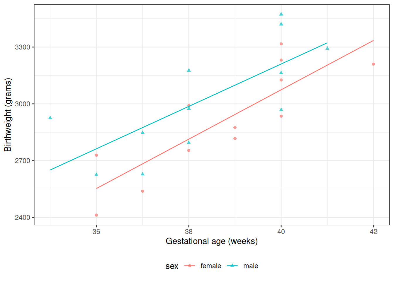
2.1 Motivating example: birthweights and gestational age
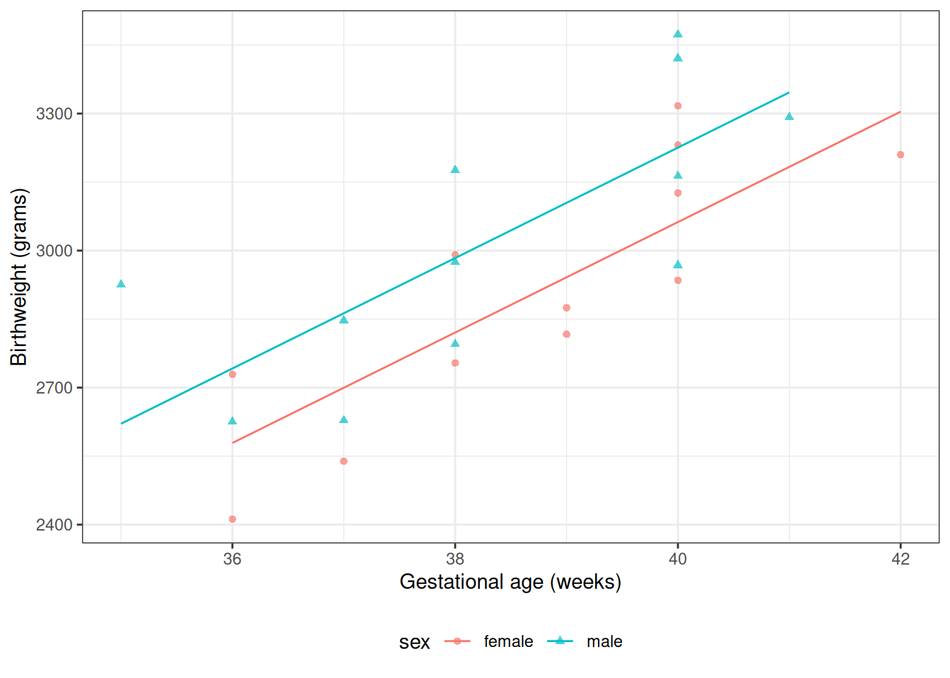
Suppose we want to learn about the distributions of birthweights (outcome\(Y\)) for (human) babies born at different gestational ages (covariate\(A\)) and with different chromosomal sexes (covariate\(S\)) (Dobson and Barnett (2018) Example 2.2.2).
pred_female <-coef(bw_lm1)["(Intercept)"] +coef(bw_lm1)["age"] *36## or using built-in prediction:pred_female_alt <-predict(bw_lm1, newdata =tibble(sex ="female", age =36))
Exercise 10 What is the interpretation of \(\beta_{M}\) in Model 2?
Solution.
Mean birthweight among males with gestational age 0 weeks: \[
\begin{aligned}
\mu(1,0) &= \text{E}{\left[Y|M = 1,A = 0\right]}\\
&= \beta_0 + {\color{red}\beta_M} \cdot 1 + \beta_A \cdot 0 + \beta_{AM}\cdot 1 \cdot 0\\
&= \beta_0 + {\color{red}\beta_M}
\end{aligned}
\] Mean birthweight among females with gestational age 0 weeks: \[
\begin{aligned}
\mu(0,0) &= \text{E}{\left[Y|M = 0,A = 0\right]}\\
&= \beta_0 + {\color{red}\beta_M} \cdot 0 + \beta_A \cdot 0 + \beta_{AM}\cdot 0 \cdot 0\\
&= \beta_0
\end{aligned}
\]
\[
\begin{aligned}
\beta_{M} &= \mu(1,0) - \mu(0,0) \\
&= \text{E}{\left[Y|M = 1,A = 0\right]} - \text{E}{\left[Y|M = 0,A = 0\right]}
\end{aligned}
\]\(\beta_M\) is the difference in mean birthweight between males with gestational age 0 weeks and females with gestational age 0 weeks.
Exercise 11 What is the interpretation of \(\beta_{AM}\) in Model 2?
Let the coefficients of this model be \(\gamma\)s instead of \(\beta\)s.
What are the interpretations of the \(\gamma\)s? How do they relate to the \(\beta\)s in Model 2? Which have the same interpretation? Which are different, and how do they differ? What is the pattern?
Solution. Interpretation of \(\gamma_0\):
From Model 4, \(\gamma_0\) is the mean birthweight among females (\(M = 0\)) with \(A^* = 0\) (i.e., \(A = 32\) weeks):
Since shifting \(A\) by a constant does not change the slope, \(\gamma_{A^*} = \beta_A\): these two coefficients have the same value and interpretation.
Interpretation of \(\gamma_{A^*M}\):
From Model 4, \(\gamma_{A^*M}\) is the difference in slope with respect to \(A^*\) between males and females:
Since shifting \(A\) by a constant does not change slopes, \(\gamma_{A^*M} = \beta_{AM}\): these two coefficients have the same value and interpretation.
The pattern:
Slope coefficients (\(\gamma_{A^*}\) and \(\gamma_{A^*M}\)) are unchanged by rescaling: they have the same values and interpretations as the corresponding \(\beta\)s.
Coefficients change only for variables that have interactions with the rescaled variable \(A\). This includes the intercept (which can be viewed as the main effect of a variable that interacts with \(A\) via \(\beta_A\)), and the main effect of \(M\) (which interacts with \(A\) via \(\beta_{AM}\)). Shifting \(A\) by 32 weeks changes the reference point from \(A = 0\) to \(A = 32\), so these coefficients now represent quantities evaluated at \(A = 32\) weeks rather than at \(A = 0\) weeks.
Exercise 13 Using R, fit the rescaled interaction model with \(A^* = A - 36\) weeks in place of \(A\) in Model 2. Compare the coefficient estimates with those from the original model. Which coefficients change, and which remain the same?
Solution.
[R code]
bw <- bw |>mutate(`age - mean`= age -mean(age),`age - 36wks`= age -36 )lm1_c <-lm(weight ~ sex +`age - 36wks`, data = bw)lm2_c <-lm(weight ~ sex +`age - 36wks`+ sex:`age - 36wks`, data = bw)parameters(lm2_c, ci_method ="wald") |>print_md()
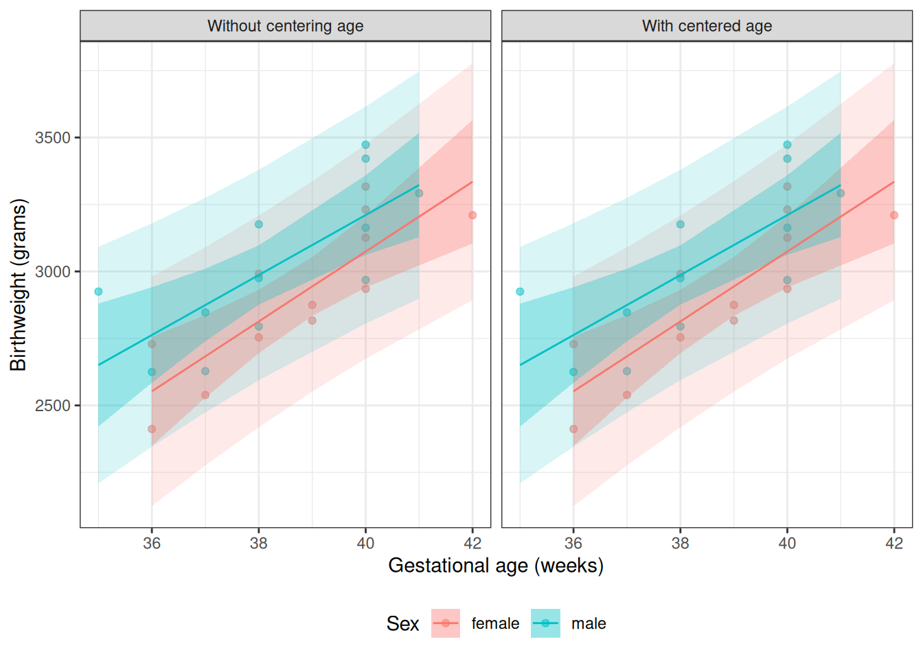
Centering gestational age does not change predictions
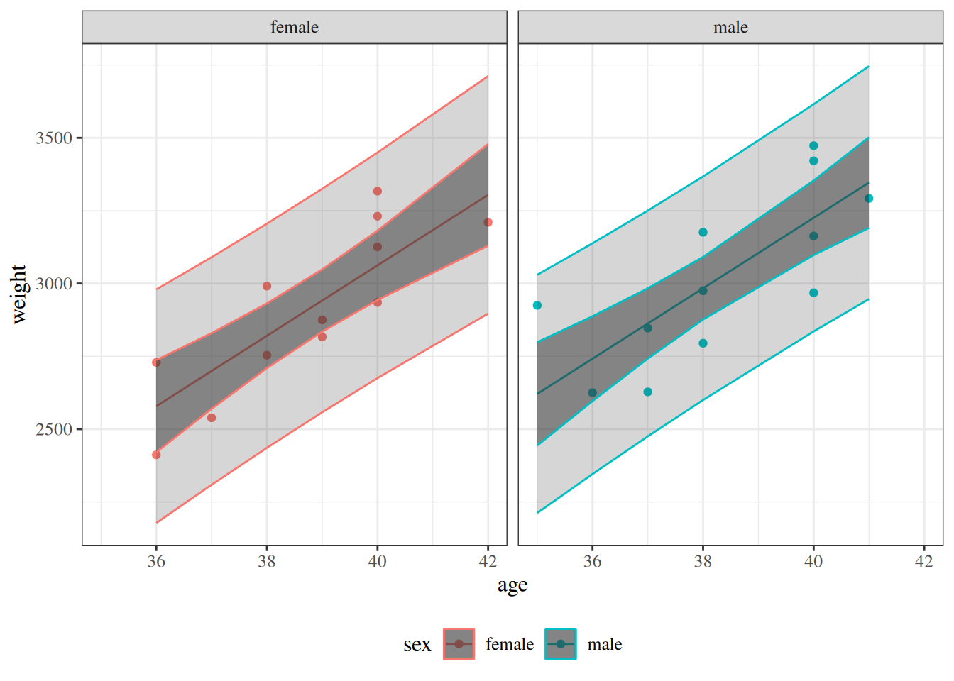
Centering gestational age changes the coefficient parameterization, but it does not change fitted values, confidence bands, or prediction bands.
The next output reports maximum absolute differences between the uncentered and centered models. All values should be near zero (up to floating-point rounding), which confirms that centering changes parameterization only.
Figure 6: Two-panel comparison of the fitted birthweight model bw_lm2 with and without centering gestational age, showing identical fitted values, confidence bands, and prediction bands in both panels.
2.8 Categorical covariates with more than two levels
Example: birthweight
In the birthweight example, the variable sex had only two observed values:
[R code]
unique(bw$sex)#> [1] female male #> Levels: female male
If there are more than two observed values, we can’t just use a single variable with 0s and 1s.
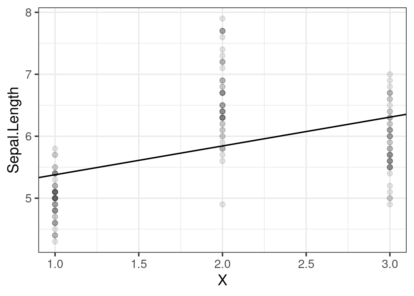
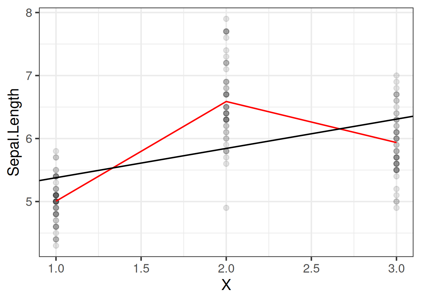
If we want to model Sepal.Length by species, we could create a variable \(X\) that represents “setosa” as \(X=1\), “virginica” as \(X=2\), and “versicolor” as \(X=3\).
[R code]
data(iris) # this step is not always necessary, but ensures you're starting# from the original version of a dataset stored in a loaded packageiris <- iris |>tibble() |>mutate(X =case_when( Species =="setosa"~1, Species =="virginica"~2, Species =="versicolor"~3 ) )iris |>distinct(Species, X)
Table 10: iris data with numeric coding of species
Then we could fit a model like:
[R code]
iris_lm1 <-lm(Sepal.Length ~ X, data = iris)iris_lm1 |>parameters() |>print_md()
Table 11: Model of iris data with numeric coding of Species
Assume the design matrix \(\mathbf{X}\) has full column rank. This implies that \(\sum_{i=1}^n \tilde{x}_i {\tilde{x}_i}^{\top}\) is invertible. To solve for \(\tilde{\beta}\), use \(\tilde{x}_i (\tilde{x}_i \cdot \tilde{\beta}) = (\tilde{x}_i {\tilde{x}_i}^{\top})\tilde{\beta}\):
\(\ell_{\beta, \beta'} ''(\beta, \sigma^2;\mathbf X,\tilde{y})\) is negative definite at \(\beta = (\mathbf{X}'\mathbf{X})^{-1}X'y\), so \(\hat \beta_{ML} = (\mathbf{X}'\mathbf{X})^{-1}X'y\) is the MLE for \(\beta\).
where \(\ell(\hat\theta)\) is the log-likelihood evaluated at the maximum-likelihood estimates \(\hat\theta\), \(p\) is the number of estimated parameters (including \(\hat\sigma^2\) for Gaussian models), and \(n\) is the number of observations.
Definition 2 (Bayesian Information Criterion (BIC))\[\text{BIC} = -2 \ell(\hat\theta) + p \log(n)\]
where \(\ell(\hat\theta)\), \(p\), and \(n\) are defined as in Definition 1.
Conceptual basis
Each criterion has two components:
Fit term (\(-2\ell(\hat\theta)\)): measures lack of fit — lower is better. A model with more parameters will always achieve a higher (or equal) log-likelihood on the observed data.
Penalty term (\(2 p\) for AIC; \(p \log(n)\) for BIC): penalizes model complexity to guard against overfitting.
Together, they balance goodness of fit against parsimony.
AIC vs. BIC
Criterion
Penalty per parameter
Tends to select
AIC
\(2\)
larger models
BIC
\(\log(n)\)
smaller models
The BIC penalty exceeds the AIC penalty whenever \(\log(n) > 2\), i.e., when \(n > e^2 \approx 7.4\). In practice, BIC almost always penalizes additional parameters more heavily than AIC and therefore tends to select simpler (more parsimonious) models (Vittinghoff et al. 2012; Kleinbaum et al. 2014).
AIC in R
[R code]
-2*logLik(bw_lm2) |>as.numeric() +2* (length(coef(bw_lm2)) +1) # sigma counts as a parameter here#> [1] 323.159AIC(bw_lm2)#> [1] 323.159
Lower values are better. There are no hypothesis tests or p-values associated with these criteria.
To compare models, calculate the criterion for each model and choose the model with the smallest value.
Differences of less than 2 units are generally considered negligible; differences greater than 10 are considered strong evidence in favor of the lower-criterion model.
BIC tends to favor simpler models than AIC, especially when the sample size is large.
(Residual) Deviance
Let \(q\) be the number of distinct covariate combinations in a data set.
For example, in the birthweight data, there are \(q = 12\) unique patterns (Table 17).
[R code]
bw_X_unique
Table 17: Unique covariate combinations in the birthweight data, with replicate counts
Definition 3 (Replicates) If a given covariate pattern has more than one observation in a dataset, those observations are called replicates.
Example 2 (Replicates in the birthweight data) In the birthweight dataset, there are 2 replicates of the combination “female, age 36” (Table 17).
Exercise 14 (Replicates in the birthweight data) Which covariate pattern(s) in the birthweight data has the most replicates?
Solution 1 (Replicates in the birthweight data). Two covariate patterns are tied for most replicates: males at age 40 weeks and females at age 40 weeks. 40 weeks is the usual length for human pregnancy (Polin et al. (2011)), so this result makes sense.
[R code]
bw_X_unique |> dplyr::filter(n ==max(n))
Saturated models
The most complicated model we could fit would have one parameter (a mean) for each covariate pattern, plus a variance parameter:
We can calculate the log-likelihood of this model as usual:
[R code]
logLik(lm_max)#> 'log Lik.' -151.402 (df=13)
We can compare this model to our other models using chi-square tests, as usual:
[R code]
library(lmtest)lrtest(lm_max, bw_lm2)
The likelihood ratio statistic for this test is \[\lambda = 2 * (\ell_{\text{full}} - \ell) = 10.355374\] where:
\(\ell_{\text{full}}\) is the log-likelihood of the full model: -151.401601
\(\ell\) is the log-likelihood of our comparison model (two slopes, two intercepts): -156.579288
This statistic is called the deviance or residual deviance for our two-slopes and two-intercepts model; it tells us how much the likelihood of that model deviates from the likelihood of the maximal model.
The corresponding p-value tells us whether there we have enough evidence to detect that our two-slopes, two-intercepts model is a worse fit for the data than the maximal model; in other words, it tells us if there’s evidence that we missed any important patterns. (Remember, a nonsignificant p-value could mean that we didn’t miss anything and a more complicated model is unnecessary, or it could mean we just don’t have enough data to tell the difference between these models.)
Null Deviance
Similarly, the least complicated model we could fit would have only one mean parameter, an intercept:
\[\text E[Y|X=x] = \beta_0\] We can fit this model in R like so:
[R code]
lm0 <-lm(weight ~1, data = bw)lm0 |>parameters() |>print_md()
Parameter
Coefficient
SE
95% CI
t(23)
p
(Intercept)
2967.67
57.58
(2848.56, 3086.77)
51.54
< .001
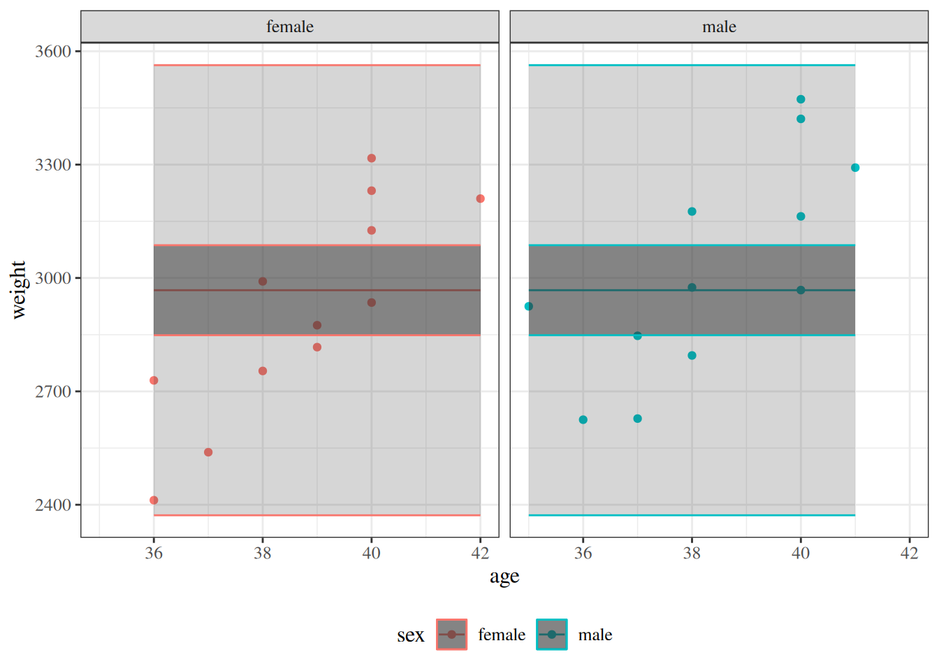
Figure 10: Null model and model 2 for birthweight data, with 95% confidence and prediction intervals.
And we can compare it to more complicated models using a likelihood ratio test:
[R code]
lrtest(bw_lm2, lm0)
The likelihood ratio statistic for the test comparing the null model to the maximal model is \[\lambda = 2 * (\ell_{\text{full}} - \ell_{0}) = 35.106732\] where:
\(\ell_{\text{0}}\) is the log-likelihood of the null model: -168.954967
\(\ell_{\text{full}}\) is the log-likelihood of the maximal model: -151.401601
In R, this test is:
[R code]
lrtest(lm_max, lm0)
This log-likelihood ratio statistic is called the null deviance. It tells us whether we have enough data to detect a difference between the null and full models.
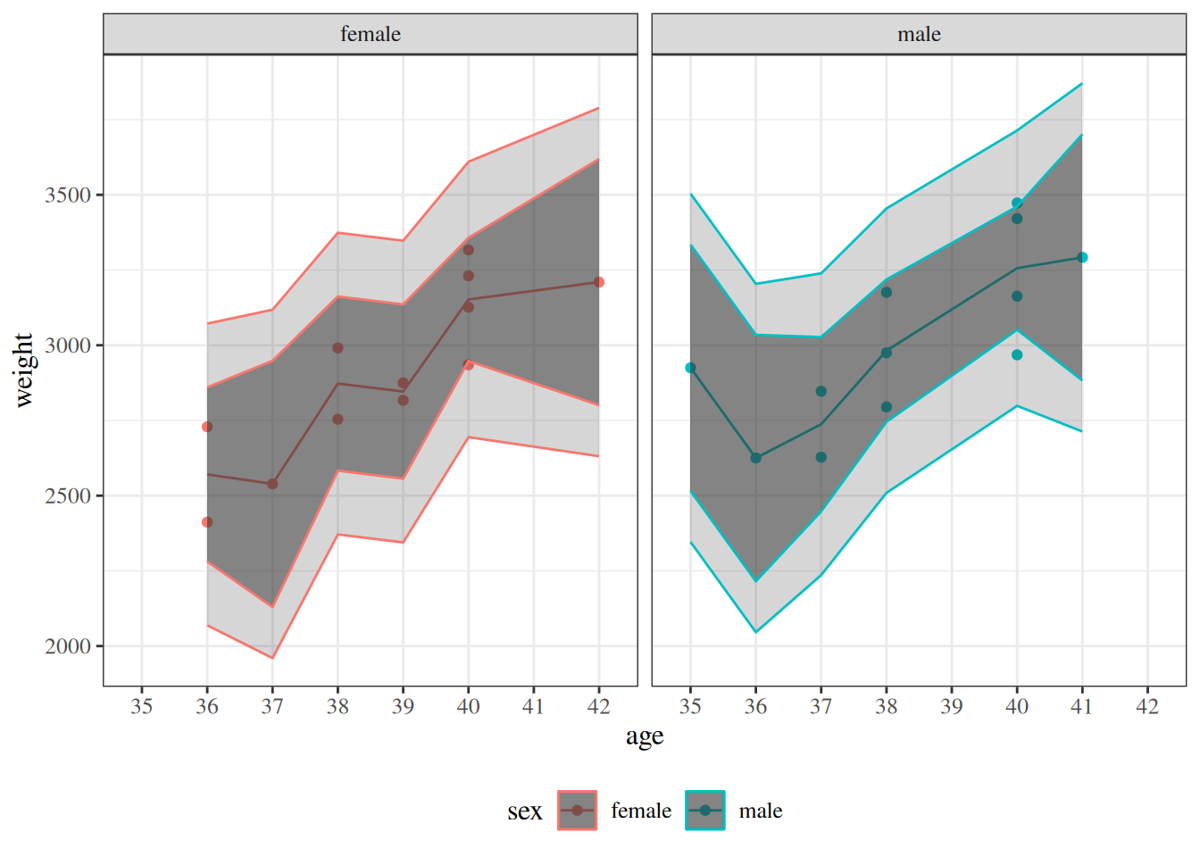
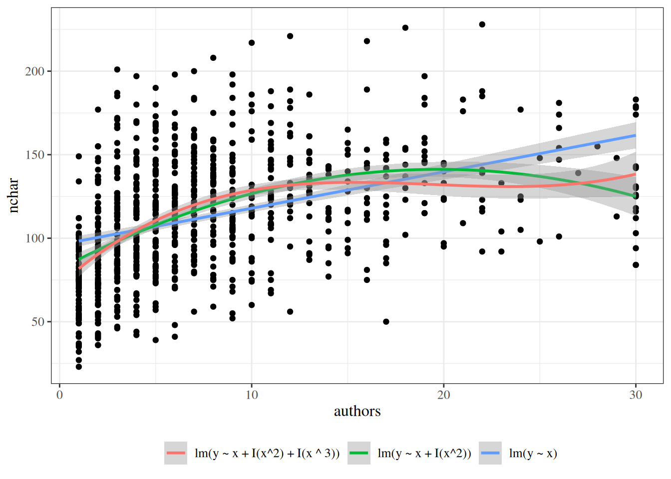
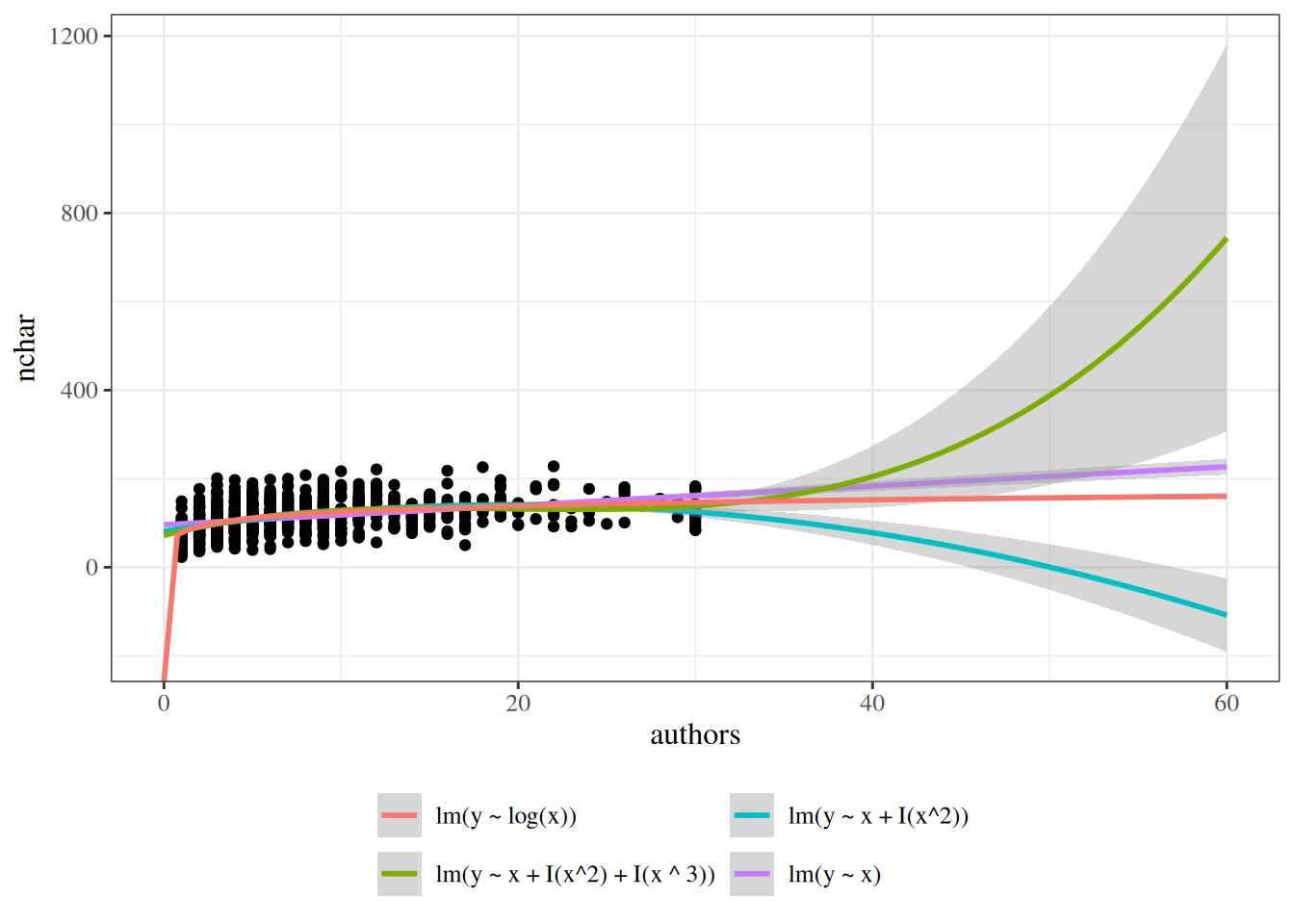
Figure 11: Four models for birthweight data, with 95% confidence and prediction intervals. The spectrum from null to saturated includes many other possible models, such as quadratic polynomial models (with or without interactions) and generalized additive models (GAMs).
where \(\ell_{\text{sat}}\) is the log-likelihood of the saturated model and \(\ell(\hat\beta)\) is the log-likelihood of the fitted model. However, this formula simplifies differently depending on the distribution family, and the resulting test statistics have different null distributions.
The saturated model has one free mean parameter per distinct covariate pattern. When there are no replicates (each covariate pattern appears exactly once), it sets \(\hat\mu_i = y_i\) for every observation, so its residual sum of squares is zero:
Because \(\sigma^2\) is unknown and must be estimated, comparing deviances between two nested Gaussian models uses an F-test, which is exact under Gaussian assumptions. Substituting \(D = \text{RSS}/\hat\sigma^2\), the \(\hat\sigma^2\) factors cancel:
For Poisson and Binomial models, the dispersion parameter \(\phi = 1\) is fixed rather than estimated. Consequently, the difference in deviances between two nested models follows an approximate \(\chi^2\) distribution:
\[D_1 - D_2 \;\dot \sim\; \chi^2_{p_2 - p_1}\]
This asymptotic result replaces the exact F-test used for Gaussian models.
Saturated vs. fully parametrized models with replicates
When some covariate patterns appear more than once (i.e., when there are replicates), it is important to distinguish between two special models:
The saturated model has one free mean parameter per distinct covariate pattern (\(q\) parameters, where \(q \leq n\) is the number of unique patterns).
The fully parametrized model has one free mean parameter per observation (\(n\) parameters).
When there are no replicates (\(q = n\)), these two coincide. When there are replicates (\(q < n\)), the saturated model constrains all observations sharing a covariate pattern to have the same mean, but places no constraint on means across different patterns. See Kleinbaum and Klein (2010) for further discussion of this distinction.
Deviance is always measured relative to the saturated model, not the fully parametrized model.
Gaussian deviance with replicates
When covariate pattern \(k\) has \(n_k\) replicates with sample mean \(\bar{y}_k\), the saturated model fits \(\hat\mu_k = \bar{y}_k\) for each pattern \(k\), so its residual sum of squares equals the within-group (pure error) SS:
This is nonzero whenever any covariate pattern has replicates with different response values. The Gaussian deviance relative to the saturated model is therefore:
R’s deviance() applied to an lm object returns the total fitted-model RSS, not the deviance relative to the saturated model. To compute the deviance relative to the saturated model, subtract the saturated model’s RSS: deviance(lm_fit) - deviance(lm_saturated).
For the birthweight data, we can verify this directly using bw_lm2 (the interaction model) and lm_max (the saturated model):
deviance(bw_lm2) # total RSS of fitted model#> [1] 652425deviance(lm_max) # within-group (pure error) SS#> [1] 423783deviance(bw_lm2) -deviance(lm_max) # lack-of-fit SS (deviance vs. saturated)#> [1] 228642
GLM deviance with replicates
For a Binomial GLM fit to data grouped by covariate pattern (with \(y_k\) events and \(n_k\) observations for pattern \(k\)), the saturated model sets \(\hat\pi_k^{\text{sat}} = y_k / n_k\) for each pattern \(k\). R’s deviance() correctly computes \(2(\ell_{\text{sat}} - \ell(\hat\beta))\) using this grouping:
When binomial data is ungrouped (individual Bernoulli observations, \(n_i = 1\)), R uses the fully parametrized model as its reference — assigning \(\hat\pi_i = y_i \in \{0, 1\}\) to each individual observation. Since each predicted probability is exactly 0 or 1, every Bernoulli likelihood contribution equals 1, and hence \(\ell_{\text{fp}} = 0\). Thus R’s deviance() returns \(-2\ell(\hat\beta)\).
We can verify this directly: observations are ungrouped Bernoulli with repeated covariate patterns (\(x \in \{0, 1\}\) appears three times each).
This reference model is the fully parametrized model (one parameter per observation), not the saturated model (one parameter per distinct covariate pattern). They coincide only when there are no repeated covariate patterns (\(q = n\)). When patterns do repeat (\(q < n\)), the saturated model sets \(\hat\pi_k = y_k/n_k\) per pattern, giving \(\ell_{\text{sat}} < 0\).
deviance() for ungrouped data cannot be used as a goodness-of-fit test against the \(\chi^2\) distribution when \(q < n\). The correct GOF statistic is \(2(\ell_{\text{sat}} - \ell(\hat\beta))\), but R’s deviance() for ungrouped data returns \(-2\ell(\hat\beta)\) (using \(\ell_{\text{fp}} = 0\)). These two quantities differ by \(-2\ell_{\text{sat}} > 0\) whenever \(q < n\). Even if each covariate pattern has many replicates (large \(n_k\)), R’s ungrouped deviance is the wrong statistic to compare against \(\chi^2(q - p)\). To obtain a valid GOF test when patterns repeat, fit the model using grouped data (one row per pattern with \(y_k\) and \(n_k\)), so that R uses the saturated model as its reference.
Definition 4 (Residual noise/deviation from the population mean) The residual noise in a probabilistic model \(p(Y)\), also known as the residual deviation of an observation from its population mean or residual for short, is the difference between an observed value \(y\) and its population mean:
Theorem 1 (Residuals in Gaussian models) If \(Y\) has a Gaussian distribution, then \(\varepsilon(Y)\) also has a Gaussian distribution, and vice versa.
Proof. Left to the reader.
Definition 5 (Residuals of a fitted model value) The residual of a fitted value \(\hat y\) (shorthand: “residual”) is its error relative to the observed data: \[
\begin{aligned}
e(\hat y) &\stackrel{\text{def}}{=}\varepsilon{\left(\hat y\right)}
\\&= y - \hat y
\end{aligned}
\]
With enough data and a correct model, the residuals will be approximately Gaussian distributed, with variance \(\sigma^2\), which we can estimate using \(\hat\sigma^2\); that is:
Hence, with enough data and a correct model, the standardized residuals will be approximately standard Gaussian; that is,
\[
r_i \ \sim_{\text{iid}}\ N(0,1)
\]
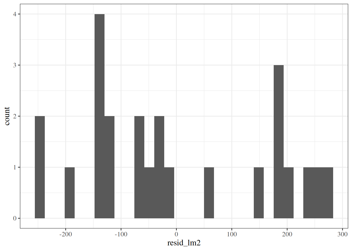
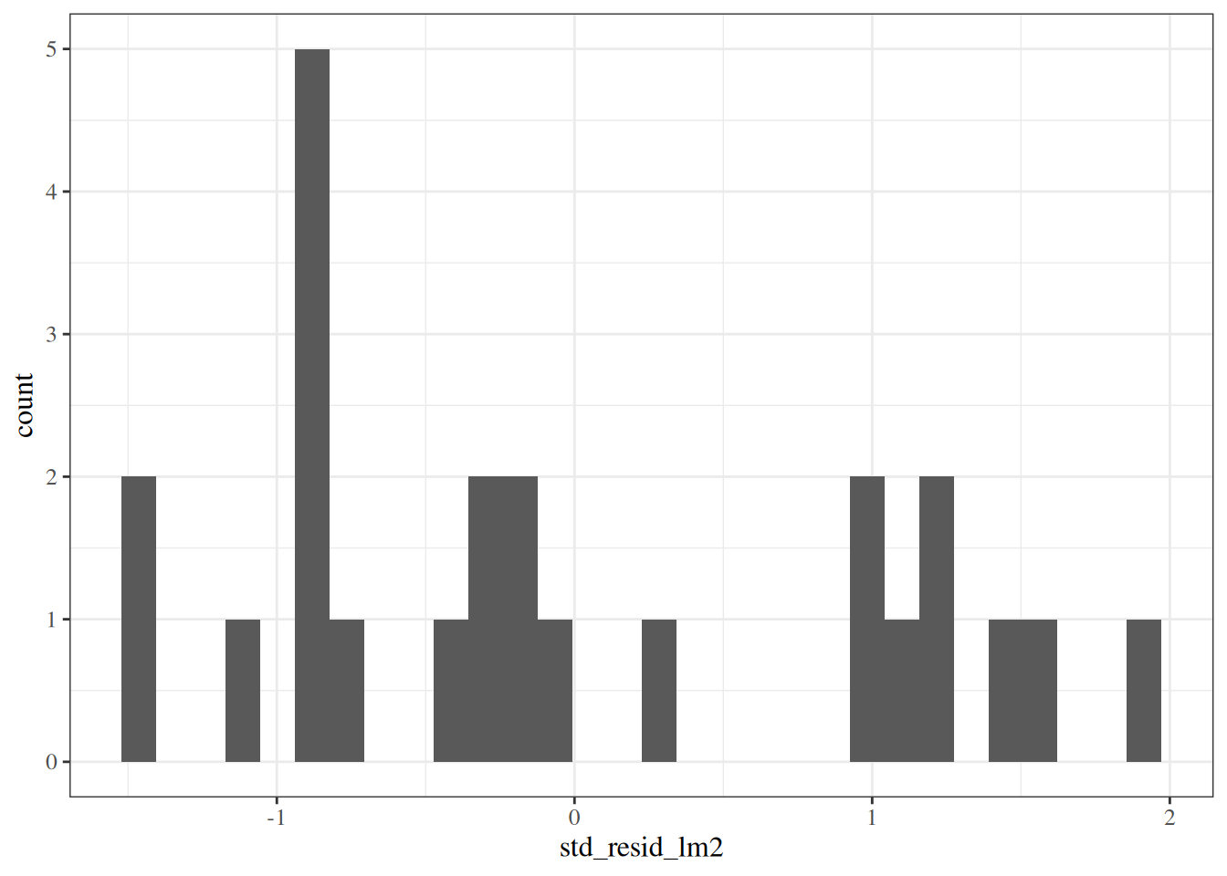
Marginal distributions of residuals
To look for problems with our model, we can check whether the residuals \(e_i\) and standardized residuals \(r_i\) look like they have the distributions that they are supposed to have, according to the model.
Figure 21: Marginal distribution of standardized residuals
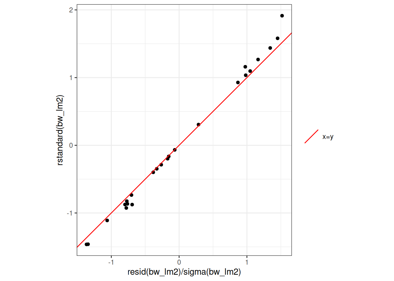
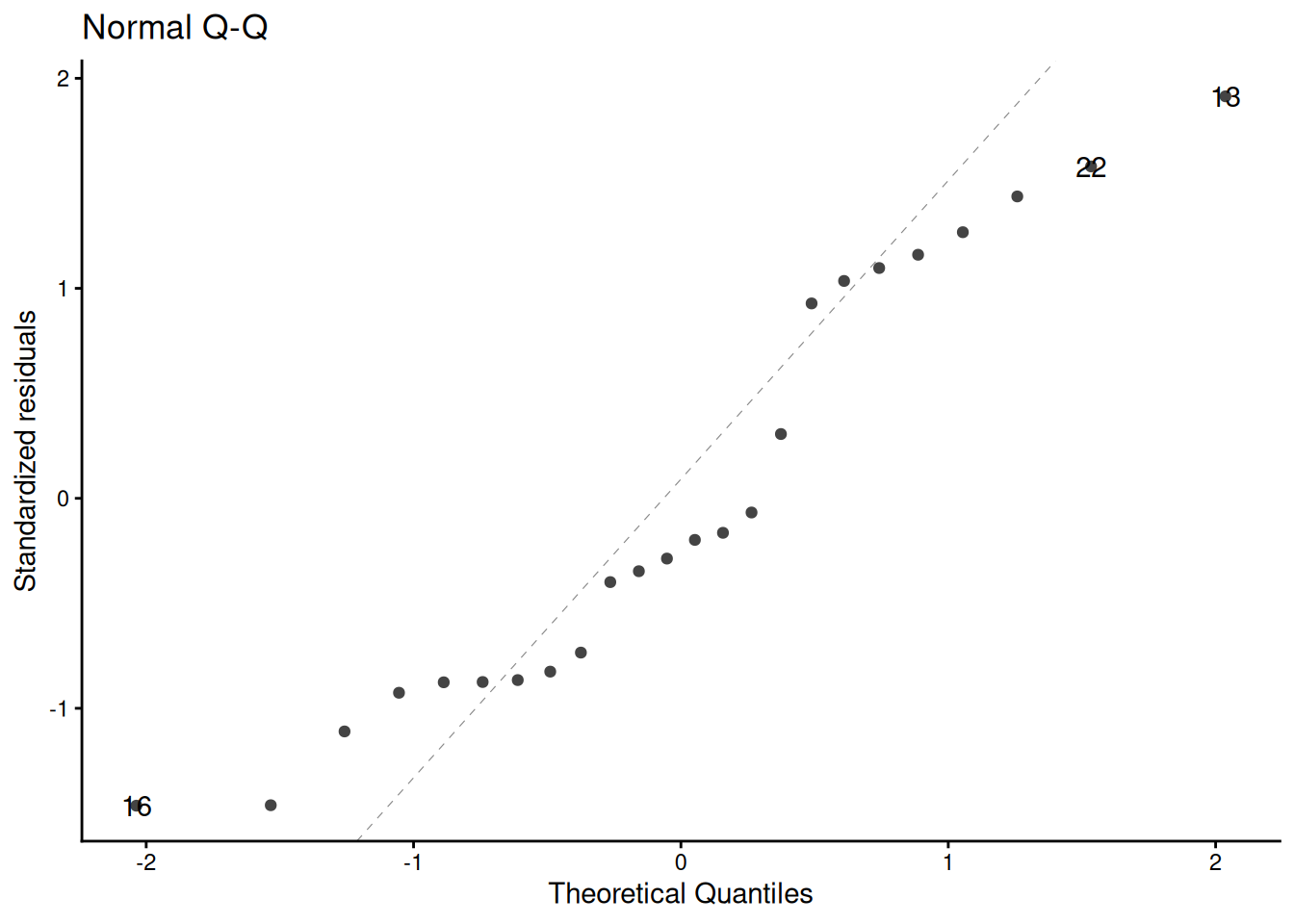
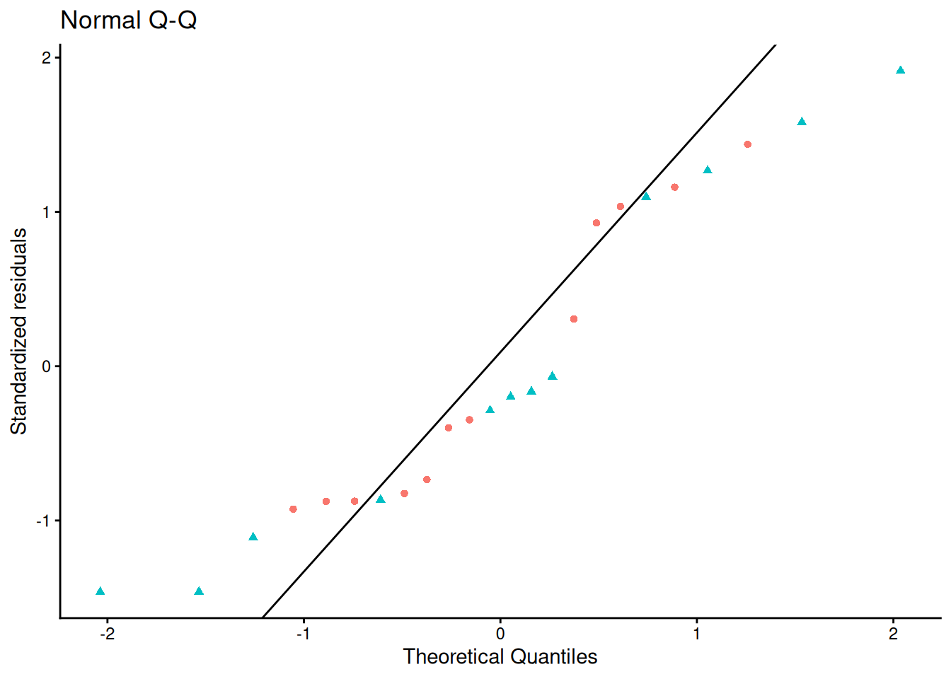
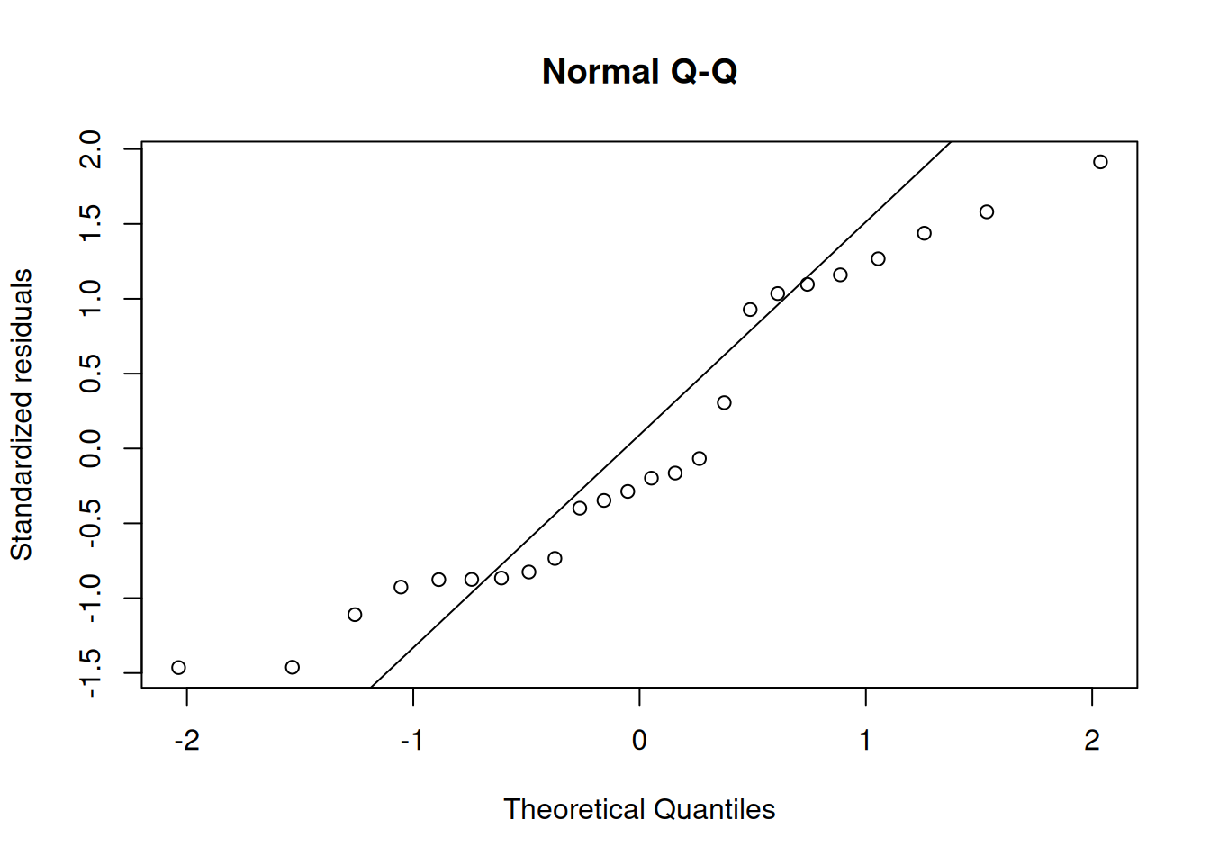
QQ plot of standardized residuals
[R code]
library(ggfortify)# needed to make ggplot2::autoplot() work for `lm` objectsqqplot_lm2_auto <- bw_lm2 |>autoplot(which =2, # options are 1:6; can do multiple at oncencol =1 ) +theme_classic()print(qqplot_lm2_auto)
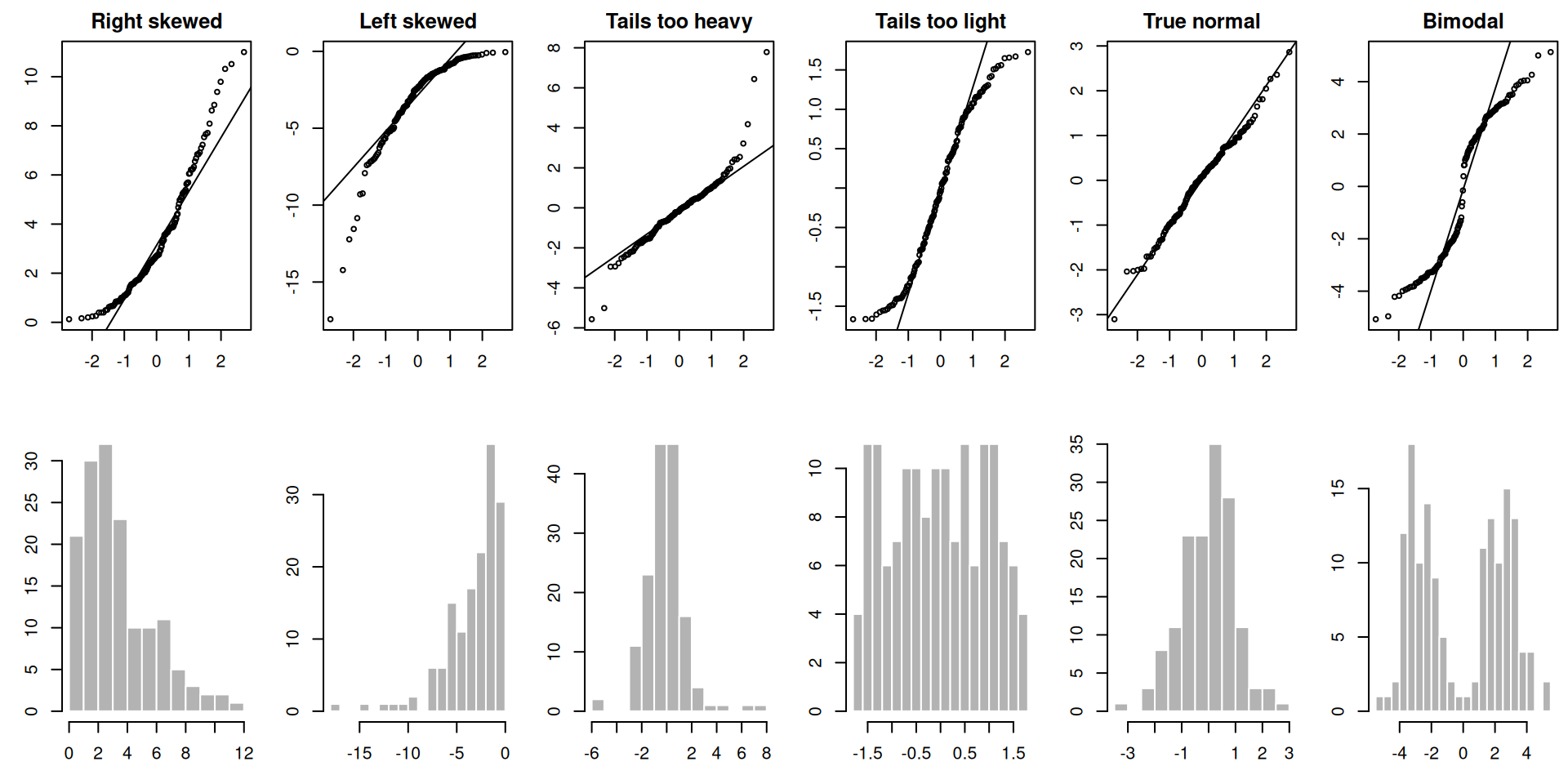
Figure 22: Typical QQ-plot patterns for six types of residual distribution. Adapted from Dunn and Smyth (2018, fig. 3.6), with thanks to the authors; reproduced here using simulated data (\(n = 150\)). Each column shows one distribution scenario: a QQ plot (top) paired with a histogram of the simulated data (bottom).
Figure 23: Three equivalent ways to produce a QQ plot of the standardized residuals for the birthweight model (Equation 2). All three plots show the same data and reference line.
Formal diagnostic tests for linear regression assumptions
Graphical diagnostics are usually the first step, but formal tests can provide numerical summaries.
For linear regression residuals, three common tests are:
fligner.test() for equal variances across groups (the Fligner–Killeen test).
Brown–Forsythe testing (a median-centered Levene variant, where standard Levene centers on group means, and Brown–Forsythe centers on group medians for more robustness; e.g., via car::leveneTest(..., center = median) or equivalent code).
Fligner–Killeen test (homoskedasticity across groups)
Suppose residuals are split into groups (\(g = 1, \ldots, G\)), for example by a categorical predictor.
The test starts from absolute deviations from each group median: \[
d_{gi} = |e_{gi} - \text{median}(e_{g1}, \ldots, e_{g,n_g})|.
\]
After ranking the pooled \(d_{gi}\) values, the Fligner–Killeen statistic is built from normal scores of those ranks.
Under the null hypothesis of equal variances, the test statistic is approximately \(\chi^2_{G-1}\). Small p-values suggest heteroskedasticity.
Levene / Brown–Forsythe test (homoskedasticity across groups)
Levene’s test transforms residuals to within-group absolute deviations: \[
z_{gi} = |e_{gi} - c_g|,
\] where \(c_g\) is the group center.
Classical Levene uses the group mean for \(c_g\). Brown–Forsythe uses the group median, which is more robust.
Then run a one-way ANOVA on \(z_{gi}\) by group: \[
F = \frac{\text{MS}_{\text{between}}}{\text{MS}_{\text{within}}}
\sim F_{G-1, N-G}
\quad\text{under }H_0.
\]
Small p-values suggest unequal residual variance.
For simple linear regression, Kutner et al. (2005, 116–17) describes the Brown–Forsythe test by splitting observations into two \(X\)-level groups (low versus high), computing absolute deviations from each group median, and applying a two-sample pooled-variance t test: let \[
z_{ij} = |e_{ij} - \tilde e_i|,
\] where \(j\) indexes observations within group \(i\), and \(\tilde e_i\) is the median residual in group \(i\). Then: \[
t_{\text{BF}} =
\frac{\bar z_{1} - \bar z_{2}}
{s_p \sqrt{1/n_{1} + 1/n_{2}}},
\quad
t_{\text{BF}} \approx t_{n_{1}+n_{2}-2}
\text{ under }H_0.
\] Here, \(\bar z_{1}\) and \(\bar z_{2}\) are the means of the \(z_{ij}\) values in groups \(i=1\) and \(i=2\), \(s_p\) is their pooled standard deviation, and \(n_{1}, n_{2}\) are the two group sample sizes. Large \(|t_{\text{BF}}|\) indicates nonconstant residual variance.
Shapiro–Wilk test (normality of standardized residuals)
For ordered standardized residuals \(r_{(1)} \le \cdots \le r_{(n)}\), the Shapiro–Wilk statistic is: \[
W =
\frac{\left(\sum_{i=1}^n a_i r_{(i)}\right)^2}
{\sum_{i=1}^n (r_i - \bar r)^2},
\] where \(a_i\) are constants from normal-order-statistic moments. The numerator uses ordered residuals \(r_{(i)}\), while the denominator uses the original (unordered) residuals.
If residuals are Gaussian, \(W\) tends to be close to 1. Small \(W\) (and small p-value) indicates departure from normality.
Interpretation rule: for all three tests, a small p-value is evidence against the corresponding model assumption.
Compared with visual diagnostics:
Fligner–Killeen / Levene summarizes the same heteroscedasticity signal that we inspect in residuals-vs-fitted (Figure 24) and scale-location (Figure 32) plots.
Shapiro–Wilk summarizes the same normality signal that we inspect in QQ plots (Figure 23 (c)) and standardized-residual histograms (Figure 21).
Use tests and plots together: the tests provide a single numerical summary, while the plots show the shape and practical size of departures.
Conditional distributions of residuals
If our Gaussian linear regression model is correct, the residuals \(e_i\) and standardized residuals \(r_i\) should have:
an approximately Gaussian distribution, with:
a mean of 0
a constant variance
This should be true for every value of \(x\).
If we didn’t correctly guess the functional form of the linear component of the mean, \[\text{E}[Y|X=x] = \beta_0 + \beta_1 X_1 + ... + \beta_p X_p\]
Then the residuals might have nonzero mean.
Regardless of whether we guessed the mean function correctly, ther the variance of the residuals might differ between values of \(x\).
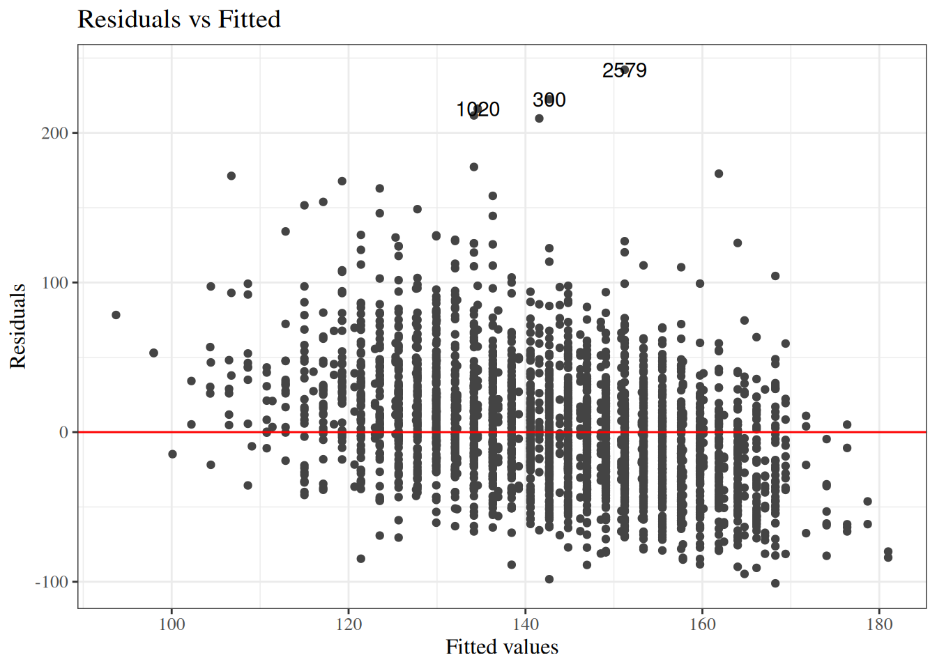
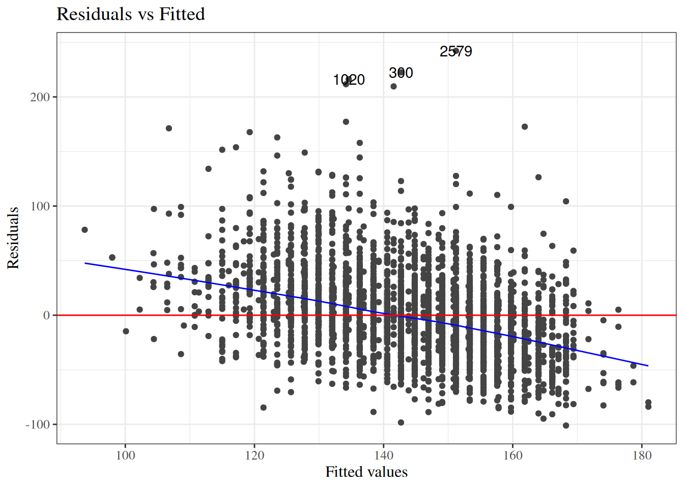
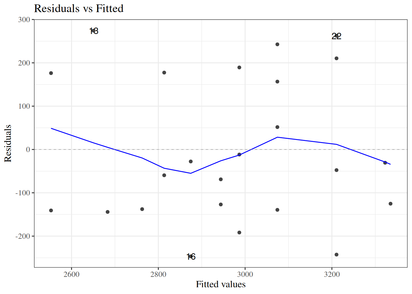
Residuals versus fitted values
[R code]
autoplot(bw_lm2, which =1, ncol =1) |>print()
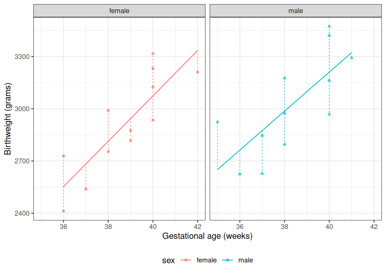
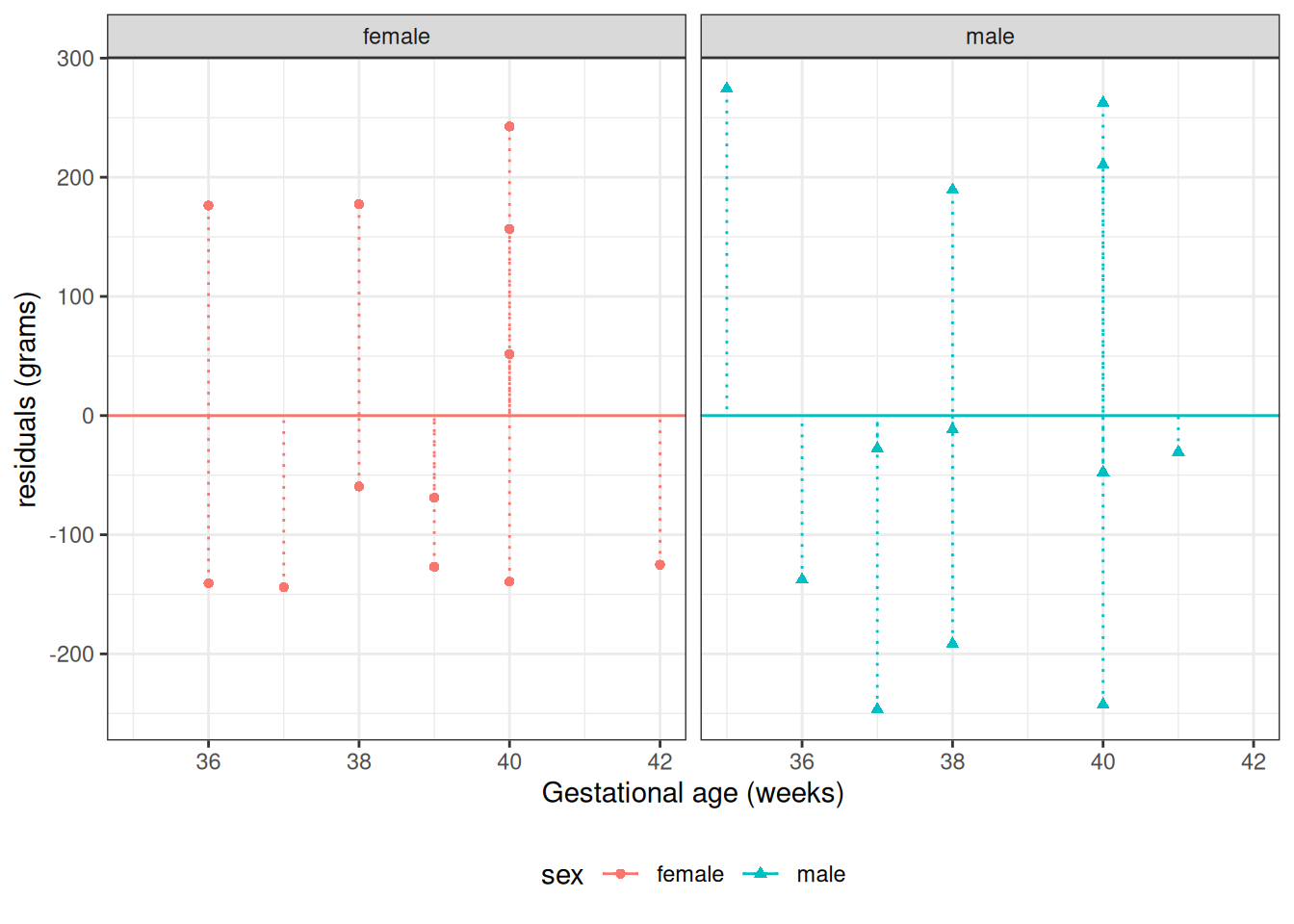
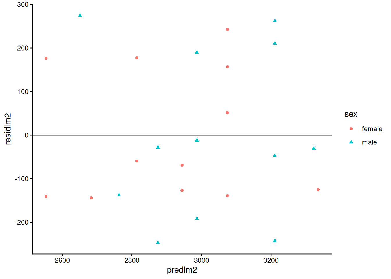
Figure 24: birthweight model (Equation 2): residuals versus fitted values
resid_vs_fit <- bw |>ggplot(aes(x = predlm2, y = residlm2, col = sex, shape = sex) ) +geom_point() +theme_classic() +geom_hline(yintercept =0)print(resid_vs_fit)
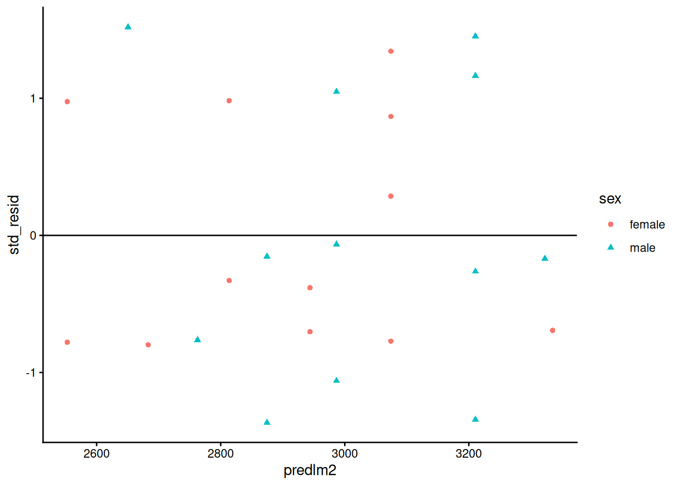
Standardized residuals vs fitted
[R code]
bw |>ggplot(aes(x = predlm2, y = std_resid, col = sex, shape = sex) ) +geom_point() +theme_classic() +geom_hline(yintercept =0)
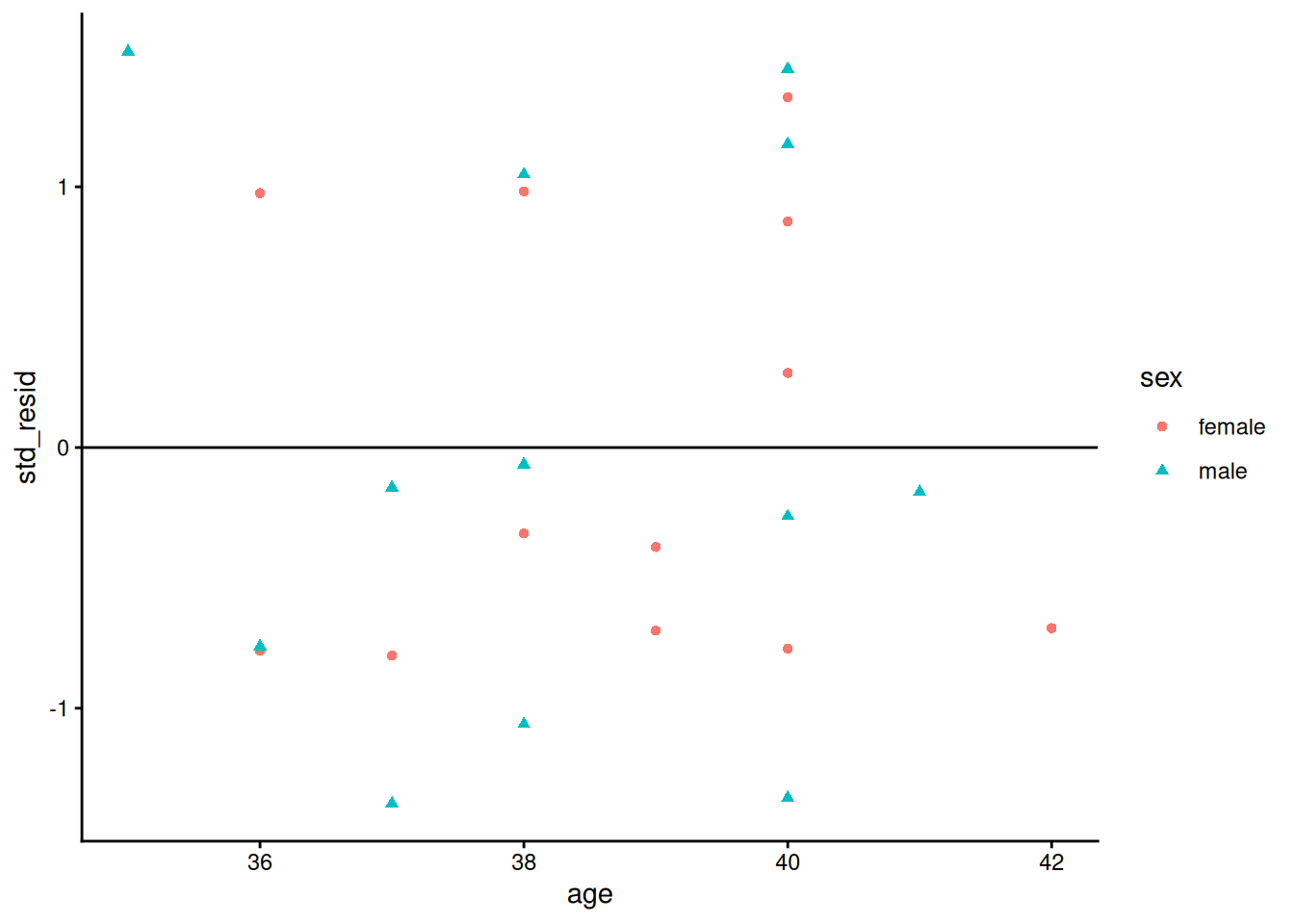
Standardized residuals vs gestational age
[R code]
bw |>ggplot(aes(x = age, y = std_resid, col = sex, shape = sex) ) +geom_point() +theme_classic() +geom_hline(yintercept =0)
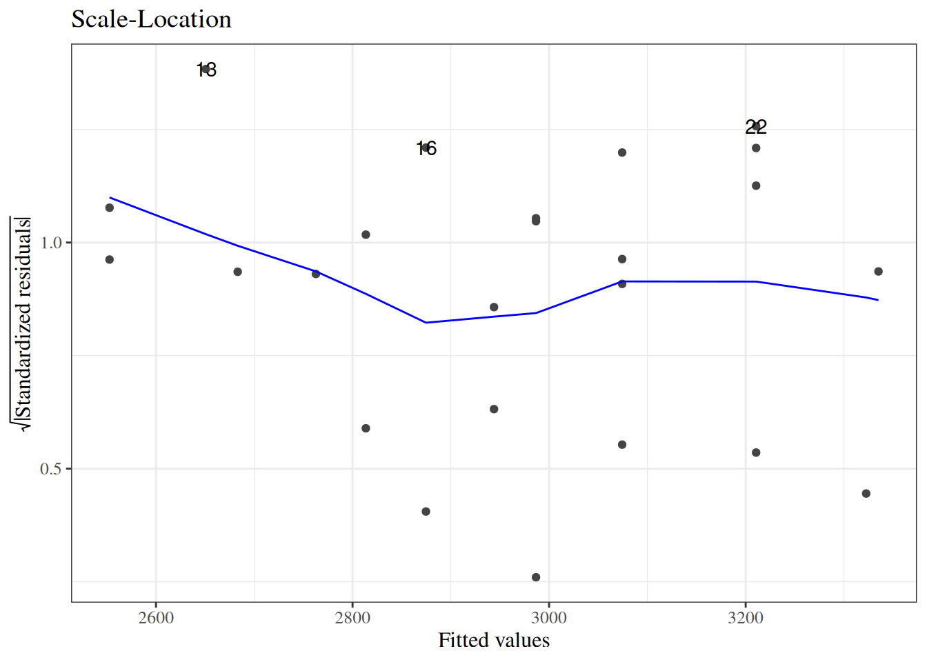
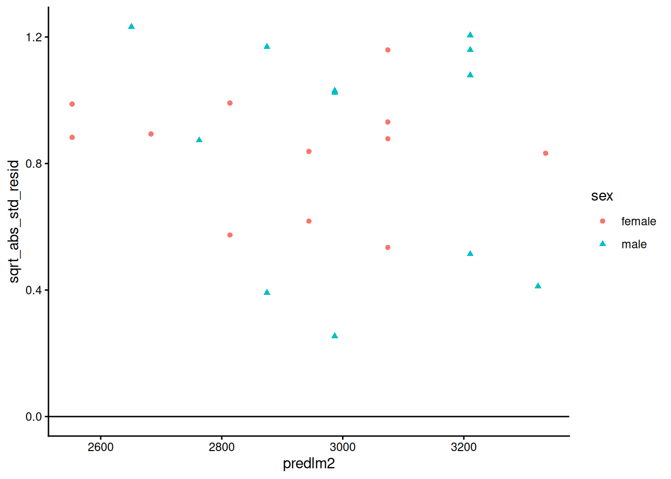
sqrt(abs(rstandard())) vs fitted
Compare with autoplot(bw_lm2, 3)
[R code]
bw |>ggplot(aes(x = predlm2, y = sqrt_abs_std_resid, col = sex, shape = sex) ) +geom_point() +theme_classic() +geom_hline(yintercept =0)
4.3 Model selection
(adapted from Dobson and Barnett (2018) §6.3.3; for more information on prediction, see James et al. (2013) and Harrell (2015)).
DAGs for variable selection
For explanatory models, variable inclusion should not rely on automated algorithms alone. Directed acyclic graphs (DAGs) can help us encode substantive assumptions about which variables are confounders, mediators, or colliders.
In a Dobson-style workflow, we use the DAG first to decide a defensible adjustment set, then compare candidate regression models within that set using predictive or likelihood-based criteria. This keeps model selection aligned with study design, rather than only with numerical fit.
Mean squared error
We might want to minimize the mean squared error, \(\text{E}{\left[(y-\hat y)^2\right]}\), for new observations that weren’t in our data set when we fit the model.
Unfortunately, \[\frac{1}{n}\sum_{i=1}^n (y_i-\hat y_i)^2\] gives a biased estimate of \(\text{E}{\left[(y-\hat y)^2\right]}\) for new data. If we want an unbiased estimate, we will have to be clever.
This is one reason that \(R^2\) is not enough for model selection. \(R^2\) does not decrease as we add explanatory variables, even when those variables do not improve out-of-sample prediction. That can lead to overfitting.
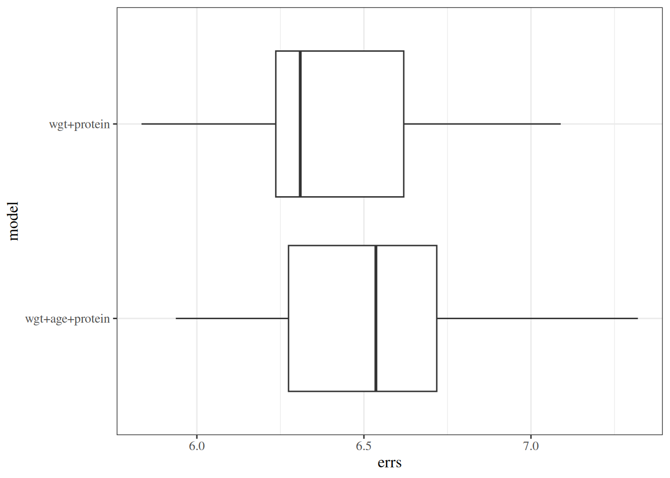
With a training/test split, we estimate coefficients in the training data and compute prediction error in held-out data:
Rather than one arbitrary split, \(k\)-fold cross-validation repeatedly partitions the data into training and test folds. For each split we compute prediction error, then summarize errors across folds and replications. The preferred model has lower prediction error, with simpler models favored when errors are similar.
When the number of candidate explanatory variables is small, we can compare all possible subsets (\(2^p\) models) using the same cross-validation metric.
[R code]
data("carbohydrate", package ="dobson")library(cvTools)full_model <-lm(carbohydrate ~ ., data = carbohydrate)cv_full <- full_model |>cvFit(data = carbohydrate, K =5, R =10,y = carbohydrate$carbohydrate )reduced_model <- full_model |>update(formula =~ . - age)cv_reduced <- reduced_model |>cvFit(data = carbohydrate, K =5, R =10,y = carbohydrate$carbohydrate )
When the number of candidate predictors is modest, we can use best subset selection. For each model size \(k = 0, 1, \ldots, p\), we fit all \(\binom{p}{k}\) models and keep the best model of size \(k\) (e.g., by lowest RSS in the training data).
This gives at most \(p+1\) candidate models to compare across model sizes, using criteria such as cross-validated prediction error, \(C_p\), AIC/BIC, or adjusted \(R^2\). In that sense, best subset selection is more exhaustive than one-path methods like forward or backward stepwise selection.
Stepwise methods are another common approach. Forward selection adds variables one at a time. Backward selection starts with the full model and removes variables sequentially. Both approaches can select different models from the same data.
Caution about stepwise selection
Stepwise regression has several known problems:
It tends to select too many variables (overfitting)
P-values and confidence intervals are biased after selection
It ignores model uncertainty
Results can be unstable across different samples
Consider using cross-validation, penalized methods (like Lasso), or subject-matter knowledge instead. See Harrell (2015) and Heinze et al. (2018) for more discussion.
[R code]
library(olsrr)olsrr:::ols_step_both_aic(full_model)#> #> #> Stepwise Summary #> -------------------------------------------------------------------------#> Step Variable AIC SBC SBIC R2 Adj. R2 #> -------------------------------------------------------------------------#> 0 Base Model 140.773 142.764 83.068 0.00000 0.00000 #> 1 protein (+) 137.950 140.937 80.438 0.21427 0.17061 #> 2 weight (+) 132.981 136.964 77.191 0.44544 0.38020 #> -------------------------------------------------------------------------#> #> Final Model Output #> ------------------#> #> Model Summary #> ---------------------------------------------------------------#> R 0.667 RMSE 5.505 #> R-Squared 0.445 MSE 30.301 #> Adj. R-Squared 0.380 Coef. Var 15.879 #> Pred R-Squared 0.236 AIC 132.981 #> MAE 4.593 SBC 136.964 #> ---------------------------------------------------------------#> RMSE: Root Mean Square Error #> MSE: Mean Square Error #> MAE: Mean Absolute Error #> AIC: Akaike Information Criteria #> SBC: Schwarz Bayesian Criteria #> #> ANOVA #> -------------------------------------------------------------------#> Sum of #> Squares DF Mean Square F Sig. #> -------------------------------------------------------------------#> Regression 486.778 2 243.389 6.827 0.0067 #> Residual 606.022 17 35.648 #> Total 1092.800 19 #> -------------------------------------------------------------------#> #> Parameter Estimates #> ----------------------------------------------------------------------------------------#> model Beta Std. Error Std. Beta t Sig lower upper #> ----------------------------------------------------------------------------------------#> (Intercept) 33.130 12.572 2.635 0.017 6.607 59.654 #> protein 1.824 0.623 0.534 2.927 0.009 0.509 3.139 #> weight -0.222 0.083 -0.486 -2.662 0.016 -0.397 -0.046 #> ----------------------------------------------------------------------------------------
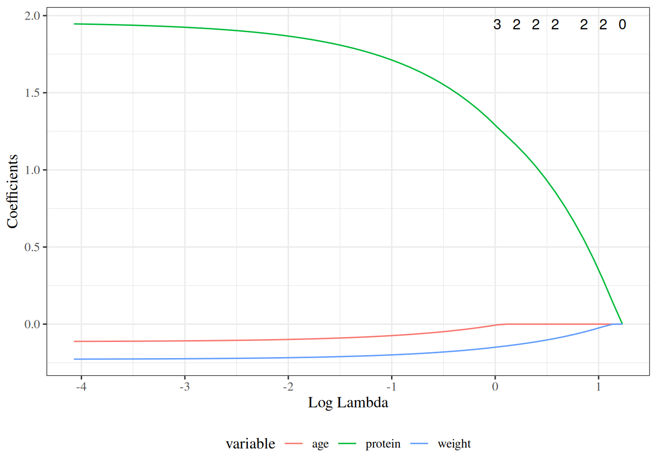
Lasso
Lasso is a penalized regression method that shrinks coefficient estimates toward zero. It adds an \(L_1\) penalty term to the objective function, creating a trade-off between model fit and parsimony. The intercept is not penalized.
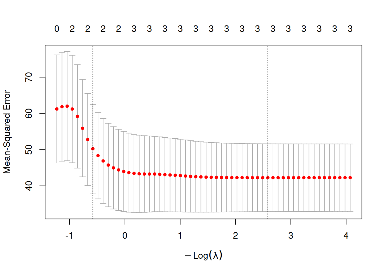
As the tuning parameter \(\lambda\) increases, more coefficients are shrunken strongly, and some become exactly zero. So lasso both regularizes the model and performs variable selection. In practice, \(\lambda\) is usually chosen by cross-validation to minimize prediction error.
For Gaussian linear models, the penalized least-squares forms are:
coef(cvfit, s ="lambda.1se")#> 4 x 1 sparse Matrix of class "dgCMatrix"#> lambda.1se#> (Intercept) 34.2044364#> age . #> weight -0.0925966#> protein 0.8582398
The reduced model (Equation 14) has \(p_1\) parameters. The full model (Equation 15) adds \(q\) extra predictors and has \(p_2 = p_1 + q\) parameters. The reduced model is a special case of the full model with the constraint \(\tilde{\gamma} = \tilde{0}\).
\(H_0: \beta_{AM} = 0\) vs. \(H_A: \beta_{AM} \neq 0\).
F-statistic
Definition 8 (Partial F-statistic) Let \(\text{RSS}_0\) and \(\text{RSS}_1\) denote the residual sums of squares from the reduced and full models, respectively. The partial F-statistic is:
\(\text{RSS}_0 = \sum_{i=1}^n(y_i - \hat{y}_i^{(0)})^2\) is the residual SS under \(H_0\)
\(\text{RSS}_1 = \sum_{i=1}^n(y_i - \hat{y}_i^{(1)})^2\) is the residual SS under \(H_A\)
\(q = p_2 - p_1\) is the number of constraints (extra parameters in the full model)
\(n - p_2\) is the residual degrees of freedom of the full model
Theorem 3 (Null distribution of the partial F-statistic) Under \(H_0\) and the Gaussian linear regression assumptions,
\[
F \ \sim \ F_{q,\; n - p_2}
\tag{17}\]
This is an exact result (not an asymptotic approximation): it holds for any sample size \(n\) when the errors \(\epsilon_i \ \sim_{\text{iid}}\ N(0, \sigma^2)\).
Proof. Under \(H_0\), the extra predictors \(\tilde{z}\) contribute nothing, so the numerator \(\text{RSS}_0 - \text{RSS}_1 \ \sim \ \sigma^2 \chi^2_q\) and the denominator \(\text{RSS}_1 \ \sim \ \sigma^2 \chi^2_{n-p_2}\) are independent chi-squared random variables (this follows from the Gauss-Markov theorem and the properties of projections in the column spaces of the design matrices). Therefore,
From Section 4.1.8, the Gaussian deviance of model \(k\) is \(D_k = \text{RSS}_k / \hat\sigma^2\), where \(\hat\sigma^2\) is an estimate of \(\sigma^2\). Because \(\hat\sigma^2\) appears in both the numerator and denominator of Equation 16, it cancels:
For Gaussian linear regression, the MLE of \(\sigma^2\) under model \(k\) is \(\hat\sigma^2_k = \text{RSS}_k / n\), so the log-likelihood at the MLE is:
So \(\lambda \approx q \cdot F\) for large \(n\), and both statistics have the same asymptotic null distribution \(\chi^2_q\) (since \(q \cdot F_{q, n-p_2} \dot \sim \chi^2_q\) as \(n \to \infty\)).
Why use the F-test instead of the LRT?
For Gaussian linear regression:
The F-test is exact — it has the correct \(F_{q,n-p_2}\) null distribution for any sample size \(n\), provided the errors are Gaussian. It accounts for the estimation of \(\sigma^2\) via the residual degrees of freedom.
The LRT is approximate — it relies on the asymptotic \(\chi^2_q\) distribution, which requires large \(n\) and treats \(\sigma^2\) as known (fixed at its MLE).
Both tests give similar p-values for large \(n\). For small to moderate \(n\), the F-test is preferred because it is exact.
For non-Gaussian GLMs (Poisson, Binomial), the F-test is not applicable; the LRT (or Wald test) is the standard approach.
In R
In R, the partial F-test for two nested lm models is performed with anova():
anova(bw_lm1, bw_lm2)
Table 23
For comparison, the approximate likelihood ratio test using the lmtest package:
lmtest::lrtest(bw_lm1, bw_lm2)
Table 24
Extracting F-test components by hand
To understand the computation, we can replicate the F-statistic manually:
Table 25
rss0 <-deviance(bw_lm1) # RSS of reduced modelrss1 <-deviance(bw_lm2) # RSS of full modeln <-nobs(bw_lm2)p2 <-length(coef(bw_lm2))q <-length(coef(bw_lm2)) -length(coef(bw_lm1))s2 <- rss1 / (n - p2) # residual variance estimate from full modelF_stat <- ((rss0 - rss1) / q) / s2p_val <-pf(F_stat, df1 = q, df2 = n - p2, lower.tail =FALSE)cat("RSS_0 =", rss0, "\n")#> RSS_0 = 658771cat("RSS_1 =", rss1, "\n")#> RSS_1 = 652425cat("q =", q, "\n")#> q = 1cat("s^2 =", s2, "\n")#> s^2 = 32621.2cat("F =", F_stat, "\n")#> F = 0.194543cat("p-val =", p_val, "\n")#> p-val = 0.663893
Table 27: Covariance matrix of \(\hat{\tilde{\beta}}\) for birthweight model 2 (with interaction term)
Interpreting the layout of the covariance matrix
The covariance matrix \(\widehat{\text{Cov}}(\hat{\tilde{\beta}})\) is a \(p \times p\) symmetric matrix, where \(p\) is the number of regression coefficients (including the intercept, if present). Its rows and columns correspond to those \(p\) coefficient estimates. When an intercept is included, the coefficients are typically written \(\hat\beta_0, \hat\beta_1, \ldots\), with \(\hat\beta_0\) denoting the intercept. The matrix entries themselves are still indexed by position, so matrix row/column index \(1\) corresponds to the intercept term when one is included.
The diagonal entries are the variances of the individual coefficient estimates: the entry in matrix position \((j+1, j+1)\) is \(\text{Var}{\left(\hat\beta_j\right)}\), for \(j = 0, 1, \ldots, p - 1\).
The off-diagonal entries are the covariances between pairs of coefficient estimates: the entry in matrix position \((i+1, j+1)\) is \(\text{Cov}{\left(\hat\beta_i, \hat\beta_j\right)}\), for \(i \neq j\).
The matrix is symmetric: \(\text{Cov}{\left(\hat\beta_i, \hat\beta_j\right)} = \text{Cov}{\left(\hat\beta_j, \hat\beta_i\right)}\).
Example 5 (Schematic for the birthweight model) For model 2, which has four coefficients \((\hat\beta_0, \hat\beta_M, \hat\beta_A, \hat\beta_{AM})\), the covariance matrix has the following layout:
Table 28: Estimated model for birthweight data with interaction term
Parameter
Coefficient
SE
95% CI
t(20)
p
(Intercept)
-2141.67
1163.60
(-4568.90, 285.56)
-1.84
0.081
sex (male)
872.99
1611.33
(-2488.18, 4234.17)
0.54
0.594
age
130.40
30.00
(67.82, 192.98)
4.35
< .001
sex (male) × age
-18.42
41.76
(-105.52, 68.68)
-0.44
0.664
Wald tests and confidence intervals
For Gaussian linear regression, the ordinary least squares (OLS) estimates \(\hat\beta_k\) are exactly Gaussian when the error terms \(\epsilon_i\) are Gaussian, for any sample size. See also the table of Gaussian vs. MLE-based tests.
Wald test statistic
To test \(H_0: \beta_k = \beta_{k,0}\) (typically \(\beta_{k,0} = 0\)):
Exercise 16 Given a maximum likelihood estimate \(\hat{\tilde{\beta}}\) and a corresponding estimated covariance matrix \(\hat \Sigma\stackrel{\text{def}}{=}\widehat{\text{Cov}}(\hat{\tilde{\beta}})\), calculate a 95% confidence interval for the predicted mean \(\mu(\tilde{x}) = \text{E}{\left[Y|\tilde{X}=\tilde{x}\right]}\).
Combining Equation 24 and the Gauss-Markov theorem:
Theorem 4 (Estimated variance and standard error of predicted mean)\[
{\color{orange}\widehat{\text{Var}}{\left(\hat\mu(\tilde{x})\right)}} = {\color{orange}{\tilde{x}}^{\top}\hat{\Sigma}\tilde{x}}
\tag{25}\]
In R, predict() with se.fit = TRUE computes the estimated mean \(\hat\mu(\tilde{x}) = \tilde{x}'\hat{\tilde{\beta}}\) and its estimated standard error for each covariate pattern:
Table 31: Predicted means and 95% CI using interval = 'confidence'
fit
lwr
upr
age
sex
2762.71
2584.34
2941.07
36
male
2986.67
2876.05
3097.29
38
male
3210.64
3062.23
3359.05
40
male
5.4 Inference for differences in means
Exercise 18 Given a maximum likelihood estimate \(\hat{\tilde{\beta}}\) and a corresponding estimated covariance matrix \(\hat \Sigma\stackrel{\text{def}}{=}\widehat{\text{Cov}}(\hat{\tilde{\beta}})\), calculate a 95% confidence interval for the difference in means comparing covariate patterns \(\tilde{x}\) and \({\tilde{x}^*}\), \(\mu(\tilde{x}) - \mu({\tilde{x}^*})\).
Combining Equation 29 and the Gauss-Markov theorem:
Theorem 5 (Estimated variance and standard error of difference in means)\[
{\color{orange}\widehat{\text{Var}}{\left(\widehat{\mu(\tilde{x}) - \mu({\tilde{x}^*})}\right)}} = {\color{orange}{\Delta\tilde{x}}^{\top}\hat{\Sigma}(\Delta\tilde{x})}
\tag{30}\]
In R, we can compute the CI for the difference in means by computing the predicted means for both covariate patterns and applying the variance formula directly:
Table 32: 95% CI for difference in birthweight means (male vs. female)
diff_mean
se
ci_lower
ci_upper
136.305
95.846
-63.626
336.236
6 Prediction
6.1 Prediction for linear models
Definition 9 (Predicted value) In a regression model \(\text{p}(y|\tilde{x})\), the predicted value of \(y\) given \(\tilde{x}\) is the estimated mean of \(Y\) given \(\tilde{X}=\tilde{x}\):
\[\hat y \stackrel{\text{def}}{=}\hat{\text{E}}{\left[Y|\tilde{X}=\tilde{x}\right]}\]
For linear models, the predicted value can be straightforwardly calculated by multiplying each predictor value \(x_j\) by its corresponding coefficient \(\beta_j\) and adding up the results:
These special predictions are called the fitted values of the dataset:
Definition 10 For a given dataset \((\tilde{Y}, \mathbf{X})\) and corresponding fitted model \(\text{p}_{\hat \beta}(\tilde{y}|\mathbf{x})\), the fitted value of \(y_i\) is the predicted value of \(y\) when \(\tilde{X}=\tilde{x}_i\) using the estimate parameters \(\hat \beta\).
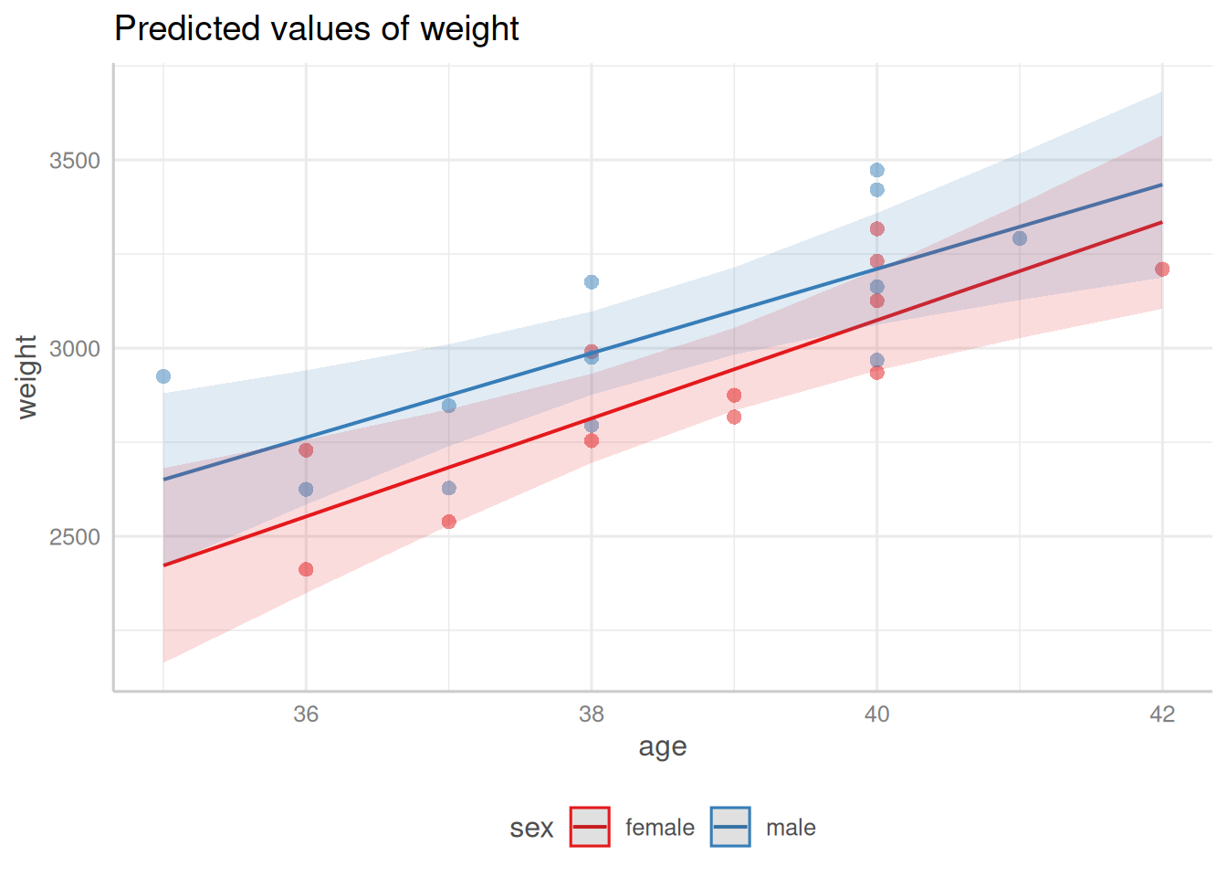
Figure 36: Predicted values and confidence bands for the birthweight model with interaction term
Why are confidence bands narrower near the center of the data?
The confidence bands in Figure 36 are visibly narrower near the center of the gestational age range. To understand why, consider a simple linear regression with one predictor \(a\) (gestational age) and an intercept. The covariate vector for a new observation at age \(a\) is \(\tilde{x}= {(1, a)}^{\top}\), and the general variance formula for the predicted mean specializes to:
where \(\bar{a} = \frac{1}{n}\sum_{i=1}^na_i\) is the mean gestational age and \(S_{AA} = \sum_{i=1}^n(a_i - \bar{a})^2\) is the total variation in gestational age.
To derive Equation 32, first note that for \(n\) observations with design matrix rows \((1, a_i)\):
Since \((a - \bar{a})^2 \geq 0\) and equals zero when \(a = \bar{a}\), the standard error is minimized at the mean gestational age \(\bar{a}\) and increases as \(a\) moves away from \(\bar{a}\) in either direction. Consequently, confidence intervals are narrowest at \(\bar{a}\) and widen toward the extremes of the gestational age range.
Intuitively, the fitted line is “anchored” at the center of the data: in simple linear regression with an intercept, the OLS fitted line passes exactly through the sample mean point \((\bar{a}, \bar{y})\), so the estimated mean at \(\bar{a}\) is relatively stable across different samples. Moving away from \(\bar{a}\), small changes in the estimated slope cause the fitted line to “pivot” around that anchor, producing larger changes in the predicted mean the further \(a\) is from \(\bar{a}\).
Additionally, there is typically more nearby data near the center of the covariate range, so we have more information about the true mean response there. Near the edges of the covariate range, there is less nearby data, leaving us less confident in our estimate of the mean response at those values.
6.4 Prediction intervals
We can also construct prediction intervals for the value of a new observation \(Y^*\), given a covariate pattern \({\tilde{x}^*}\).
A new observation \(Y^*\) at \({\tilde{x}^*}\) follows the same linear model as the training data:
\(\text{Var}{\left(\varepsilon^*\right)} = \sigma^2\): the variance of the future observation’s own noise, which is irreducible.
\(\text{Var}{\left({({\tilde{x}^*})}^{\top}\hat \beta\right)} = {({\tilde{x}^*})}^{\top}\text{Var}{\left(\hat \beta\right)}{\tilde{x}^*}\): the variance due to estimating the mean \({({\tilde{x}^*})}^{\top}\tilde{\beta}\) from the data.
The first component is not present in the confidence interval for \(\hat\mu({\tilde{x}^*})\), which only accounts for estimation uncertainty. This is why prediction intervals are always wider than the corresponding confidence intervals: a prediction interval must additionally account for the irreducible noise \(\varepsilon^*\) in a new observation.
The standard error of the prediction error is the square root of its variance:
Since \(\varepsilon^* \sim \text{N}{\left(0, \sigma^2\right)}\) and \(\hat \beta\sim \text{N}{\left(\tilde{\beta}, \sigma^2(\mathbf{X}'\mathbf{X})^{-1}\right)}\) are both normally distributed, and since \(\varepsilon^* \perp\!\!\!\perp\hat \beta\) (as noted above in the variance derivation), their difference \(Y^* - \hat{Y}^* = \varepsilon^* - {({\tilde{x}^*})}^{\top}(\hat \beta- \tilde{\beta})\) is also normally distributed, with mean 0 (as shown above) and variance given by Equation 34. Standardizing by dividing by \(\sigma\sqrt{1 + {({\tilde{x}^*})}^{\top}(\mathbf{X}'\mathbf{X})^{-1}{\tilde{x}^*}}\) yields a standard normal random variable. Replacing \(\sigma\) with \(\hat \sigma\), which is estimated with \(n-p\) degrees of freedom and is independent of \(Y^* - \hat{Y}^*\), the standardized prediction error follows a \(t\) distribution:
bw_lm2 |>predict(interval ="predict") |>head()#> Warning in predict.lm(bw_lm2, interval = "predict"): predictions on current data refer to _future_ responses#> fit lwr upr#> 1 2552.73 2124.50 2980.97#> 2 2552.73 2124.50 2980.97#> 3 2683.13 2275.99 3090.27#> 4 2813.53 2418.60 3208.47#> 5 2813.53 2418.60 3208.47#> 6 2943.93 2551.48 3336.38
The warning from the last command is: “predictions on current data refer to future responses” (since you already know what happened to the current data, and thus don’t need to predict it).
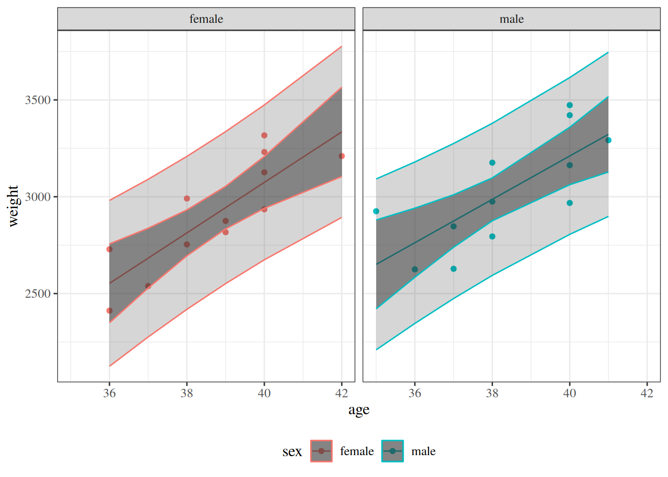
Figure 37: Confidence and prediction intervals for birthweight model 2
References
Akaike, Hirotugu. 1974. “A New Look at the Statistical Model Identification.”IEEE Transactions on Automatic Control 19 (6): 716–23. https://doi.org/10.1109/TAC.1974.1100705.
Anderson, Edgar. 1935. “The Irises of the Gaspe Peninsula.”Bulletin of American Iris Society 59: 2–5.
Harrell, Frank E. 2015. Regression Modeling Strategies: With Applications to Linear Models, Logistic Regression, and Survival Analysis. 2nd ed. Springer. https://doi.org/10.1007/978-3-319-19425-7.
Heinze, Georg, Christine Wallisch, and Daniela Dunkler. 2018. “Variable Selection – A Review and Recommendations for the Practicing Statistician.”Biometrical Journal 60 (3): 431–49. https://doi.org/10.1002/bimj.201700067.
Hogg, Robert V., Elliot A. Tanis, and Dale L. Zimmerman. 2015. Probability and Statistical Inference. Ninth edition. Pearson.
Hulley, Stephen, Deborah Grady, Trudy Bush, et al. 1998. “Randomized Trial of Estrogen Plus Progestin for Secondary Prevention of Coronary Heart Disease in Postmenopausal Women.”JAMA : The Journal of the American Medical Association (Chicago, IL) 280 (7): 605–13.
James, Gareth, Daniela Witten, Trevor Hastie, Robert Tibshirani, et al. 2013. An Introduction to Statistical Learning. Vol. 112. Springer. https://www.statlearning.com/.
Vittinghoff, Eric, David V Glidden, Stephen C Shiboski, and Charles E McCulloch. 2012. Regression Methods in Biostatistics: Linear, Logistic, Survival, and Repeated Measures Models. 2nd ed. Springer. https://doi.org/10.1007/978-1-4614-1353-0.
Weisberg, Sanford. 2005. Applied Linear Regression. Vol. 528. John Wiley & Sons.