Models for Binary Outcomes

Logistic regression and variations

Configuring R

Functions from these packages will be used throughout this document:

library(conflicted) # check for conflicting function definitions
# library(printr) # inserts help-file output into markdown output
library(rmarkdown) # Convert R Markdown documents into a variety of formats.
library(pander) # format tables for markdown
library(ggplot2) # graphics
library(ggfortify) # help with graphics
library(dplyr) # manipulate data
library(tibble) # `tibble`s extend `data.frame`s
library(magrittr) # `%>%` and other additional piping tools
library(haven) # import Stata files
library(knitr) # format R output for markdown
library(tidyr) # Tools to help to create tidy data
library(plotly) # interactive graphics
library(dobson) # datasets from Dobson and Barnett 2018
library(parameters) # format model output tables for markdown
library(haven) # import Stata files
library(latex2exp) # use LaTeX in R code (for figures and tables)
library(fs) # filesystem path manipulations
library(survival) # survival analysis
library(survminer) # survival analysis graphics
library(KMsurv) # datasets from Klein and Moeschberger
library(parameters) # format model output tables for
library(webshot2) # convert interactive content to static for pdf
library(forcats) # functions for categorical variables ("factors")
library(stringr) # functions for dealing with strings
library(lubridate) # functions for dealing with dates and times

Here are some R settings I use in this document:

rm(list = ls()) # delete any data that's already loaded into R

conflicts_prefer(dplyr::filter)
ggplot2::theme_set(
  ggplot2::theme_bw() + 
        # ggplot2::labs(col = "") +
    ggplot2::theme(
      legend.position = "bottom",
      text = ggplot2::element_text(size = 12, family = "serif")))

knitr::opts_chunk$set(message = FALSE)
options('digits' = 6)

panderOptions("big.mark", ",")
pander::panderOptions("table.emphasize.rownames", FALSE)
pander::panderOptions("table.split.table", Inf)
conflicts_prefer(dplyr::filter) # use the `filter()` function from dplyr() by default
legend_text_size = 9
run_graphs = TRUE

options(digits = 6)

Acknowledgements

This content is adapted from:

• Dobson and Barnett (2018), Chapter 7
• Vittinghoff et al. (2012), Chapter 5
• David Rocke’s materials from the 2021 edition of Epi 204
• Nahhas (2024) Chapter 6

1 Introduction

Exercise 1 What is logistic regression?

Solution 1.

Definition 1 Logistic regression is a framework for modeling binary outcomes, conditional on one or more predictors (a.k.a. covariates).

Exercise 2 (Examples of binary outcomes) What are some examples of binary outcomes in the health sciences?

Solution 2. Examples of binary outcomes include:

• exposure (exposed vs unexposed)
• disease (diseased vs healthy)
• recovery (recovered vs unrecovered)
• relapse (relapse vs remission)
• return to hospital (returned vs not)
• vital status (dead vs alive)

Logistic regression uses the Bernoulli distribution to model the outcome variable, conditional on one or more covariates.

Exercise 3 Write down a mathematical definition of the Bernoulli distribution.

Solution 3. The Bernoulli distribution family for a random variable \(X\) is defined as:

\[ \begin{aligned} \Pr(X=x) &= \text{1}_{x\in {\left\{0,1\right\}}}\pi^x(1-\pi)^{1-x}\\ &= \left\{{\pi, x=1}\atop{1-\pi, x=0}\right. \end{aligned} \]

Logistic regression versus linear regression

Logistic regression differs from linear regression, which uses the Gaussian (“normal”) distribution to model the outcome variable, conditional on the covariates.

Exercise 4 Recall: what kinds of outcomes is linear regression used for?

Solution 4. Linear regression is typically used for numerical outcomes that aren’t event counts or waiting times for an event.

Examples of outcomes that are often analyzed using linear regression include:

• weight
• height
• income
• prices

1.1 Risk estimation and prediction

In Epi 203, you have already seen methods for modeling binary outcomes using one covariate that is also binary (such as exposure/non-exposure). In this section, we review one-covariate analyses, with a special focus on risk ratios and odds ratios, which are important concepts for interpreting logistic regression.

Example 1 (Oral Contraceptive Use and Heart Attack)  

• Research question: how does oral contraceptive (OC) use affect the risk of myocardial infarction (MI; a.k.a. heart attack)?

This was an issue when oral contraceptives were first developed, because the original formulations used higher concentrations of hormones. Modern OCs don’t have this issue.

Table 1 contains simulated data for an imaginary follow-up (a.k.a. prospective) study in which two groups are identified, one using OCs and another not using OCs, and both groups are tracked for three years to determine how many in each groups have MIs.

library(dplyr)
oc_mi <-
  tribble(
    ~OC, ~MI, ~Total,
    "OC use", 13, 5000,
    "No OC use", 7, 10000
  ) |>
  mutate(`No MI` = Total - MI) |>
  relocate(`No MI`, .after = MI)

totals <-
  oc_mi |>
  summarize(across(c(MI, `No MI`, Total), sum)) |>
  mutate(OC = "Total")

tbl_oc_mi <- bind_rows(oc_mi, totals)

tbl_oc_mi |> pander::pander()

Table 1: Simulated data from study of oral contraceptive use and heart attack risk

OC	MI	No MI	Total
OC use	13	4,987	5,000
No OC use	7	9,993	10,000
Total	20	14,980	15,000

Exercise 5 Estimate the probabilities of MI for OC users and non-OC users in Example 1.

Solution 5. \[\hat{\text{p}}(MI|OC) = \frac{13}{5000} = 0.0026\]

\[\hat{\text{p}}(MI|\neg OC) = \frac{7}{10000} = 7\times 10^{-4}\]

Exercise 6 What does the term “controls” mean in the context of study design?

Solution 6.

Definition 2 (Two meanings of “controls”) Depending on context, “controls” can mean either:

• individuals who don’t experience an exposure of interest,
• or individuals who don’t experience an outcome of interest.

Exercise 7 What types of studies do the two definitions of controls correspond to?

Solution 7.

Definition 3 (cases and controls in retrospective studies) In retrospective case-control studies, participants who experience the outcome of interest are called cases, while participants who don’t experience that outcome are called controls.

Definition 4 (treatment groups and control groups in prospective studies) In prospective studies, the group of participants who experience the treatment or exposure of interest is called the treatment group, while the participants who receive the baseline or comparison treatment (for example, clinical trial participants who receive a placebo or a standard-of-care treatment rather than an experimental treatment) are called controls.

1.2 Comparing probabilities

Risk differences

The simplest comparison of two probabilities, \(\pi_1\), and \(\pi_2\), is the difference of their values:

Definition 5 (Risk difference) The risk difference of two probabilities, \(\pi_1\), and \(\pi_2\), is the difference of their values: \[\delta(\pi_1,\pi_2) \stackrel{\text{def}}{=}\pi_1 - \pi_2\]

Example 2 (Difference in MI risk) In Example 1, the maximum likelihood estimate of the difference in MI risk between OC users and OC non-users is:

\[ \begin{aligned} \hat\delta(\pi(OC), \pi(\neg OC)) &= \delta(\hat\pi(OC), \hat\pi(\neg OC))\\ &= \hat\pi(OC) - \hat\pi(\neg OC)\\ &= 0.0026 - 7\times 10^{-4}\\ &= 0.0019 \end{aligned} \]

Exercise 8 (interpreting risk differences) How can we interpret the preceding relative risk estimate in prose?

Solution 8 (interpreting risk differences). “The difference in risk of MI between OC users and non-users was 0.0019.”

or

“The difference in risk of MI between OC users and non-users was 0.19 percentage points.”

See the note about working with percentages in the Appendix.

Risk ratios

Exercise 9 If \(\pi_1\) and \(\pi_2\) are two probabilities, what do we call the following ratio?

\[\rho(\pi_1,\pi_2) = \frac{\pi_1}{\pi_2}\]

Solution 9.

Definition 6 (Relative risk ratios) The ratio of two probabilities \(\pi_1\) and \(\pi_2\),

\[\rho(\pi_1,\pi_2) = \frac{\pi_1}{\pi_2}\]

is called the:

• risk ratio,
• relative risk ratio,
• probability ratio,
• or rate ratio

of \(\pi_1\) compared to \(\pi_2\).

Exercise 10  

Above, we estimated that:

\[\hat{\text{p}}(MI|OC) = 0.0026\]

\[\hat{\text{p}}(MI|\neg OC) = 7\times 10^{-4}\]

Now, estimate the relative risk of MI for OC versus non-OC.

Solution 10.

The relative risk of MI for OC versus non-OC is:

rr <- (13 / 5000) / (7 / 10000)

\[ \begin{aligned} \hat\rho(OC, \neg OC) &=\frac{\hat{\text{p}}(MI|OC)}{\hat{\text{p}}(MI|\neg OC)}\\ &= \frac{0.0026}{7\times 10^{-4}}\\ &= 3.714286 \end{aligned} \]

Exercise 11 How can we interpret the preceding relative risk estimate in prose?

Solution 11.

We might summarize this result by saying that:

• “The estimated probability of MI among OC users was 3.714286 times as high as the estimated probability among OC non-users.”

or

• “The estimated probability of MI among OC users was 2.714286 times higher than, the estimated probability among OC non-users.”

see also Section 8.1.4 which uses similar phrasing.

Relative risk differences

The second approach above, where we subtract 1 from the risk ratio, is actually reporting a slightly different metric:

Definition 7 (Relative risk difference)  

Sometimes, we divide the risk difference by the comparison probability; the result is called the relative risk difference:

\[\xi(\pi_1,\pi_2) \stackrel{\text{def}}{=}\frac{\delta(\pi_1,\pi_2)}{\pi_2}\]

Theorem 1 (Relative risk difference equals risk ratio minus 1) \[\xi(\pi_1,\pi_2) = \rho(\pi_1,\pi_2) - 1\]

Proof. \[ \begin{aligned} \xi(\pi_1,\pi_2) &\stackrel{\text{def}}{=}\frac{\delta(\pi_1,\pi_2)}{\pi_2} \\&= \frac{\pi_1-\pi_2}{\pi_2} \\&= \frac{\pi_1}{\pi_2} - 1 \\&= \rho(\pi_1,\pi_2) - 1 \end{aligned} \]

Changing reference groups in risk comparisons

Risk differences, risk ratios, and relative risk differences are defined by two probabilities, plus a choice of which probability is the baseline or reference probability (i.e., which probability is the subtrahend of the risk difference or the denominator of the risk ratio).

\[\delta(\pi_2,\pi_1) = -\delta(\pi_1, \pi_2)\]

\[\rho(\pi_2,\pi_1) = {\left(\rho(\pi_1,\pi_2)\right)}^{-1}\] \[\xi(\pi_2,\pi_1) = {\left(\xi(\pi_1,\pi_2) + 1\right)}^{-1} - 1\]

Exercise 12 Prove the relationships above.

Example 3 (Switching the reference group in a risk ratio) Above, we estimated that the risk ratio of OC versus non-OC is:

\[ \begin{aligned} \rho(OC, \neg OC) &= 3.714286 \end{aligned} \]

In comparison, the risk ratio for non-OC versus OC is:

\[ \begin{aligned} \rho(\neg OC, OC) &=\frac{\hat{\text{p}}(MI|\neg OC)}{\hat{\text{p}}(MI|OC)}\\ &= \frac{7\times 10^{-4}}{0.0026}\\ &= 0.269231\\ &= \frac{1}{\rho(OC, \neg OC)} \end{aligned} \]

1.3 Odds and odds ratios

Odds and probabilities

In logistic regression, we will make use of a mathematically-convenient transformation of probability, called odds:

Definition 8 (Odds)  

The odds of an event \(A\), is the probability that the event occurs, divided by the probability that it doesn’t occur. We can represent odds with the Greek letter \(\omega\) (“omega”). ¹ Thus, in mathematical notation:

\[\omega\stackrel{\text{def}}{=}\frac{\Pr(A)}{\Pr(\neg A)} \tag{1}\]

1. The name “omega” is a contraction of “o mega”, which means “long o” in Greek, in contrast with “omicron” (\(\omicron\), “short o”). See https://www.etymonline.com/search?q=omega and https://en.wikipedia.org/wiki/Omega for more details.

This course is about regression models, which are conditional probability models (regression models). Accordingly, we define conditional odds in terms of conditional probabilities:

Definition 9 (Conditional odds)  

The conditional odds of an event \(A\) given a condition \(B\), is the (conditional) probability that event \(A\) occurs (given condition \(B\)), divided by the (conditional) probability that it doesn’t occur (given condition \(B\)). We can represent conditional odds using \(\omega(A|B)\), \(\omega(B)\) or \(\omega_B\) (“omega bee”). Thus, in mathematical notation:

\[\omega(B) \stackrel{\text{def}}{=}\frac{\Pr(A|B)}{\Pr(\neg A|B)} \tag{2}\]

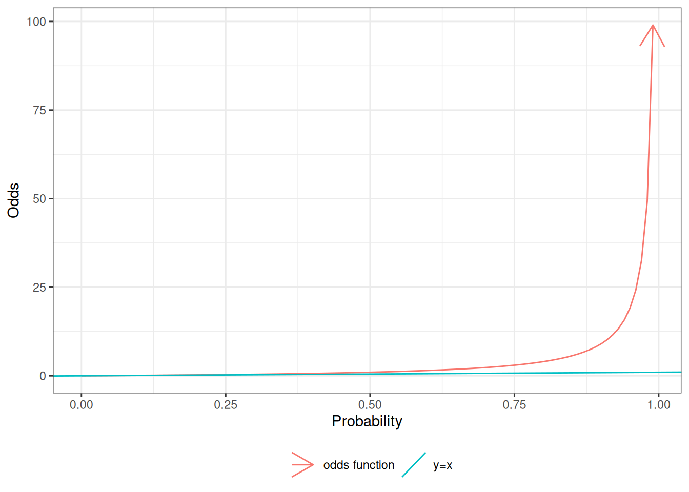
Example 4 (Computing odds from probabilities) In Exercise 5, we estimated that the probability of MI, given OC use, is \(\pi(OC) \stackrel{\text{def}}{=}\Pr(MI|OC) = 0.0026\). If this estimate is correct, then the odds of MI, given OC use, is:

\[ \begin{aligned} \omega(OC) &\stackrel{\text{def}}{=}\frac{\Pr(MI|OC)}{\Pr(\neg MI|OC)}\\ &=\frac{\Pr(MI|OC)}{1-\Pr(MI|OC)}\\ &=\frac{\pi(OC)}{1-\pi(OC)}\\ &=\frac{0.0026}{1-0.0026}\\ &\approx 0.002607 \end{aligned} \]

Exercise 13 (Computing odds from probabilities) Estimate the odds of MI, for non-OC users.

Solution. \[ \omega(\neg OC) = 7.004903\times 10^{-4} \]

Exercise 14 Find a general formula for converting probabilities into odds.

Solution 12. Using Definition 8 and the complementary probability:

\[ \begin{aligned} \omega&\stackrel{\text{def}}{=}\frac{\Pr(A)}{\Pr(\neg A)} \\ &= \frac{\pi}{1-\pi} \end{aligned} \]

Theorem 2 If \(\pi\) is the probability of an event \(A\) and \(\omega\) is the corresponding odds of \(A\), then:

\[\omega= \frac{\pi}{1-\pi} \tag{3}\]

Proof. By Solution 12.

The mathematical relationship between odds \(\omega\) and probabilities \(\pi\), which is represented in Equation 3, is a core component of logistic regression models, as we will see in the rest of this chapter. Let’s give the expression on the righthand side of Equation 3 its own name and symbol, so that we can refer to it concisely:

Definition 10 (Odds function) The odds function is defined as: \[\text{odds}{\left\{\pi\right\}} \stackrel{\text{def}}{=}\frac{\pi}{1-\pi} \tag{4}\]

We can use the odds function (Definition 10) to simplify Equation 3 (in Theorem 2) into a more concise expression, which is easier to remember and manipulate:

Corollary 1 If \(\pi\) is the probability of an outcome \(A\) and \(\omega\) is the corresponding odds of \(A\), then:

\[\omega= \text{odds}{\left\{\pi\right\}} \tag{5}\]

In other words, the odds function rescales probabilities into odds.

Proof. By Theorem 2 and Definition 10.

Exercise 15 Graph the odds function.

Solution 13.

Figure 1 graphs the odds function.

odds <- function(pi) pi / (1 - pi)
library(ggplot2)
ggplot() +
  geom_function(
    fun = odds,
    arrow = arrow(ends = "last"),
    mapping = aes(col = "odds function")
  ) +
  xlim(0, .99) +
  xlab("Probability") +
  ylab("Odds") +
  geom_abline(aes(
    intercept = 0,
    slope = 1,
    col = "y=x"
  )) +
  theme_bw() +
  labs(colour = "") +
  theme(legend.position = "bottom")

Figure 1: Odds versus probability

Theorem 3 (One-sample MLE for odds) Let \(X_1,...X_n\) be a set of \(n\) \(\text{iid}\) Bernoulli trials, and let \(X = \sum_{i=1}^nX_i\) be their sum.

Then the maximum likelihood estimate of the odds of \(X=1\), \(\omega\), is:

\[ \hat{\omega}= \frac{x}{n-x} \]

Proof. \[ \begin{aligned} 1-\hat\pi &= 1-\frac{x}{n}\\ &= \frac{n}{n} - \frac{x}{n}\\ &= \frac{n - x}{n} \end{aligned} \]

Thus, the estimated odds is:

\[ \begin{aligned} \frac{\hat\pi}{1-\hat\pi} &= \frac{\left(\frac{x}{n}\right)}{\left(\frac{n-x}{n}\right)}\\ &= \frac{x}{n-x} \end{aligned} \tag{6}\]

That is, the odds estimate can be computed directly as “# events” divided by “# nonevents”, without needing to compute \(\hat\pi\) and \(1-\hat\pi\) first.

Example 5 (Calculating odds using the shortcut) In Example 4, we calculated \[ \begin{aligned} \omega(OC) &=0.002607 \end{aligned} \]

Let’s recalculate this result using our shortcut.

Solution 14. \[ \begin{aligned} \omega(OC) &=\frac{13}{5000-13}\\ &=0.002607 \end{aligned} \]

Same answer as in Example 4!

Theorem 4 (Simplified expressions for odds function)  

Two equivalent expressions for the odds function are:

\[ \begin{aligned} \text{odds}{\left\{\pi\right\}} &= \frac{1}{\pi^{-1}-1} \\ &= {\left(\pi^{-1}-1\right)}^{-1} \end{aligned} \tag{7}\]

Exercise 16 Prove Theorem 4.

Solution 15. Starting from Definition 10:

\[ \begin{aligned} \text{odds}{\left\{\pi\right\}} &= \frac{\pi}{1-\pi} \\ &= \frac{\pi}{1-\pi}\frac{\pi^{-1}}{\pi^{-1}} \\ &= \frac{\pi\pi^{-1}}{(1-\pi)\pi^{-1}} \\ &= \frac{1}{(\pi^{-1}-\pi\pi^{-1})} \\ &= \frac{1}{(\pi^{-1}-1)} \\ &= {\left(\pi^{-1}-1\right)}^{-1} \end{aligned} \]

Corollary 2 (Odds of a non-event) If \(\pi\) is the odds of event \(A\) and \(\omega\) is the corresponding odds of \(A\), then the odds of \(\neg A\) are:

\[ \begin{aligned} \omega(\neg A) &= \frac{1-\pi}{\pi} \\&= \pi^{-1}-1 \end{aligned} \]

Proof. Left to the reader.

Odds of rare events

Exercise 17 What odds value corresponds to the probability \(\pi = 0.2\), and what is the numerical difference between these two values?

Solution. \[ \omega= \frac{\pi}{1-\pi} =\frac{.2}{.8} = .25 \]

Exercise 18 Find the difference between an odds \(\omega\) and its corresponding probability \(\pi\), as a function of \(\pi\).

Solution 16. \[ \begin{aligned} \omega- \pi &= \frac{\pi}{1-\pi} - \pi \\ &= \frac{\pi}{1-\pi} - \frac{\pi(1-\pi)}{1-\pi} \\ &= \frac{\pi}{1-\pi} - \frac{\pi - \pi^2}{1-\pi} \\ &= \frac{\pi - (\pi - \pi^2)}{1-\pi} \\ &= \frac{\pi - \pi + \pi^2}{1-\pi} \\ &= \frac{\pi^2}{1-\pi} \\ &= \frac{\pi}{1-\pi} \pi \\ &= \omega\pi \end{aligned} \]

Theorem 5 Let \(\omega= \frac{\pi}{1-\pi}\). Then:

\[\omega- \pi = \frac{\pi^2}{1-\pi}\]

Proof. By Solution 16.

For rare events (small \(\pi\)), odds and probabilities are nearly equal (see Figure 1), because \(1-\pi \approx 1\) and \(\pi^2 \approx 0\).

For example, in Example 4, the probability and odds differ by \(6.777622\times 10^{-6}\).

The inverse odds function

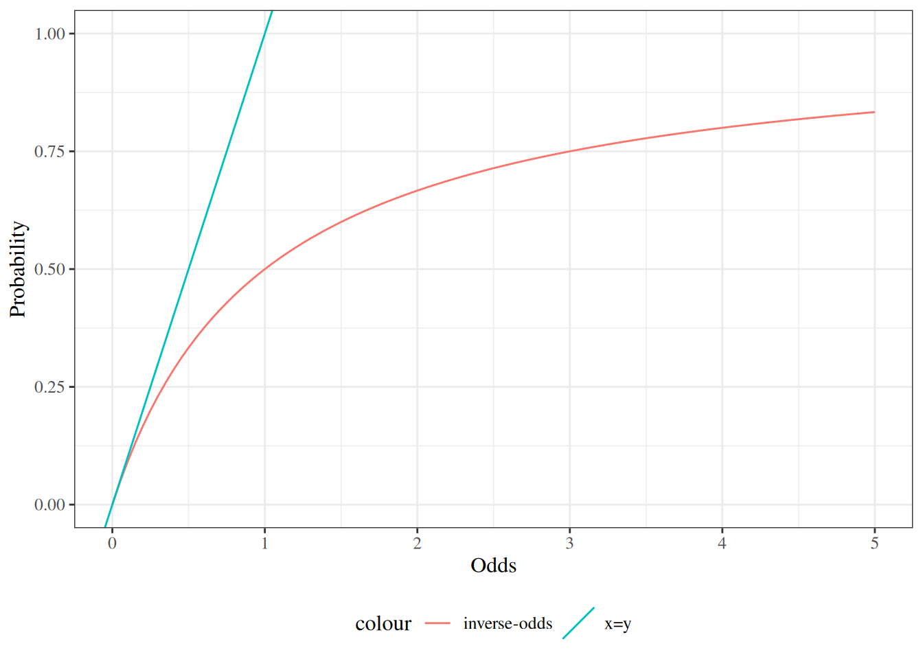
Exercise 19 If \(\pi\) is the probability of an event \(A\) and \(\omega\) is the corresponding odds of \(A\), how can we compute \(\pi\) from \(\omega\)?

For example, if \(\omega= 3/2\), what is \(\pi\)?

Solution 17. Starting from Theorem 2, we can solve Equation 3 for \(\pi\) in terms of \(\omega\):

\[ \begin{aligned} \omega&= \frac{\pi}{1-\pi} \\ (1-\pi) \omega&= \pi \\ \omega-\pi\omega&= \pi \\ \omega&= \pi + \pi\omega \\ \omega&= (1 + \omega)\pi \\ \pi &= \frac{\omega}{1 + \omega} \end{aligned} \] So if \(\omega= 3/2\),

\[ \begin{aligned} \pi &= \frac{3/2}{1 + 3/2} \\ &= \frac{3/2}{5/2} \\ &= \frac{3}{5} \end{aligned} \]

Theorem 6 If \(\pi\) is the probability of an event and \(\omega\) is the corresponding odds of that event, then:

\[\pi = \frac{\omega}{1+\omega} \tag{8}\]

Proof. By Theorem 2 and Solution 17.

Definition 11 (inverse odds function) \[ \text{invodds}{\left\{\omega\right\}} \stackrel{\text{def}}{=}\frac{\omega}{1 + \omega} \tag{9}\]

can be called the inverse-odds function.

Corollary 3 \[\pi= \text{invodds}{\left\{\omega\right\}}\]

Proof. By Definition 11 and Theorem 6.

Corollary 4 \[\text{invodds}{\left\{\omega\right\}} = \text{odds}^{-1}{\left\{\omega\right\}}\]

Proof. Using Corollary 1 and Theorem 6:

\[ \begin{aligned} \text{invodds}{\left\{\text{odds}{\left\{\pi\right\}}\right\}} &= \text{invodds}{\left\{\omega\right\}} \\ &= \frac {\omega} {1 + \omega} \\ &= \pi \end{aligned} \]

Likewise (not shown):

\[\text{odds}{\left\{\text{invodds}{\left\{\omega\right\}}\right\}} = \omega\]

The inverse-odds function converts odds into their corresponding probabilities (Figure 2). Its domain of inputs is \(\omega \in [0,\infty)\) and its range of outputs is \(\pi \in [0,1]\).

I haven’t seen anyone give the inverse-odds function a concise name; maybe \(\text{prob}()\) or \(\text{prob}()\) or \(\text{risk}()\)?

odds_inv <- function(omega) (1 + omega^-1)^-1
library(ggplot2)
ggplot() +
  geom_function(fun = odds_inv, aes(col = "inverse-odds")) +
  xlab("Odds") +
  ylab("Probability") +
  xlim(0, 5) +
  ylim(0, 1) +
  geom_abline(aes(intercept = 0, slope = 1, col = "x=y"))

Figure 2: The inverse odds function, \(\text{invodds}{\left\{\omega\right\}}\)

Exercise 20 What probability corresponds to an odds of \(\omega= 1\), and what is the numerical difference between these two values?

Solution. \[ \begin{aligned} \pi &= \text{invodds}{\left\{1\right\}} \\ &= \frac{1}{1+1} \\ &=\frac{1}{2} \\ &= .5 \end{aligned} \] \[ \begin{aligned} \omega- \pi&= 1 - .5 \\ &= .5 \end{aligned} \]

Lemma 1 (Simplified expression for inverse odds function)  

Equivalent expressions for the inverse odds function are:

\[ \begin{aligned} \text{invodds}{\left\{\omega\right\}} &= \frac{1}{1+\omega^{-1}} \\ &= (1+\omega^{-1})^{-1} \end{aligned} \tag{10}\]

Exercise 21 Prove that Equation 10 is equivalent to Definition 11.

Solution 18. Analogous to Solution 15.

Lemma 2 (One minus inverse-odds) \[1 - \pi= \frac{1}{1+\omega}\]

Proof. By Theorem 6:

\[ \begin{aligned} 1 - \pi&= 1 - \frac{\omega}{1 + \omega} \\ &= \frac{{\color{red}1+\omega}}{1 + \omega} - \frac{{\color{blue}\omega}}{1 + \omega} \\ &= \frac{{\color{red}(1+\omega)} - {\color{blue}\omega}}{1 + \omega} \\ &= \frac{1 + \omega- \omega}{1 + \omega} \\ &= \frac{1}{1 + \omega} \end{aligned} \]

Corollary 5 \[1+\omega= \frac{1}{1-\pi}\]

Odds ratios

Now that we have defined odds, we can introduce another way of comparing event probabilities: odds ratios.

Definition 12 (Odds ratio) The odds ratio for two conditional odds, \(\omega_1\) and \(\omega_2\), is the ratio of those odds:

\[\theta(\omega_1, \omega_2) \stackrel{\text{def}}{=}\frac{\omega_1}{\omega_2}\]

There’s a 1:1 mapping between probability and odds, and according to that mapping, the odds are equal between two covariate patterns IF and ONLY IF the probabilities are also equal between those patterns. So, testing whether an odds ratio = 1 is equivalent to testing whether the corresponding risk ratio = 1, and also equivalent to testing whether the risk difference = 0. Therefore, in hypothesis testing, if the null hypothesis is no effect, then we can shift between RD, RR, and OR. But when we’re talking about point estimates and CIs, we need to limit our conclusions to the effect measure(s) that we actually estimated, because the sizes of RDs, RRs, and ORs don’t have a simple relationship to each other, except when pi_1=pi_2 (as shown by Figure 3).

An odds ratio is a ratio of odds. An odds is a ratio of probabilities, so odds ratios are ratios of ratios:

Theorem 7 \[ \begin{aligned} \theta(\omega_1, \omega_2) &= \frac{\omega_1}{\omega_2} \\ &= \frac{{\left(\frac{\pi_1}{1-\pi_1}\right)}}{{\left(\frac{\pi_2}{1-\pi_2}\right)}} \end{aligned} \]

Example 6 (Calculating odds ratios) In Example 1, the odds ratio for OC users versus OC-non-users is:

\[ \begin{aligned} \theta(\omega(OC), \omega(\neg OC)) &= \frac{\omega(OC)}{\omega(\neg OC)}\\ &= \frac{0.0026}{7\times 10^{-4}}\\ &= 3.714286\\ \end{aligned} \]

A shortcut for calculating odds ratio estimates

The general form of a two-by-two table is shown in Table 2.

Table 2: A generic 2x2 table

	Event	Non-Event	Total
Exposed	a	b	a+b
Non-exposed	c	d	c+d
Total	a+c	b+d	a+b+c+d

From this table, we have:

• \(\hat\pi(Event|Exposed) = a/(a+b)\)

• \(\hat\pi(\neg Event|Exposed) = b/(a+b)\)

• \(\hat\omega(Event|Exposed) = \frac{\frac{a}{a+b}}{\frac{b}{a+b}}=\frac{a}{b}\)

• \(\hat\omega(Event|\neg Exposed) = \frac{c}{d}\) (see Exercise 22)

• \(\theta(Exposed,\neg Exposed) = \frac{\frac{a}{b}}{\frac{c}{d}} = \frac{ad}{bc}\)

Exercise 22 Given Table 2, show that \(\hat\omega(Event|\neg Exposed) = \frac{c}{d}\).

Properties of odds ratios

Odds ratios have a special property: we can swap a covariate with the outcome, and the odds ratio remains the same.

Theorem 8 (Odds ratios are reversible) For any two events \(A\), \(B\):

\[\theta(A|B) = \theta(B|A)\]

Proof. \[ \begin{aligned} \theta(A|B) &\stackrel{\text{def}}{=}\frac{\omega(A|B)}{\omega(A|\neg B)} \\ &= \frac {{\left(\frac{\text{p}(A|B)}{\text{p}(\neg A|B)}\right)}} {{\left(\frac{\text{p}(A|\neg B)}{\text{p}(\neg A| \neg B)}\right)}} \\ &= {\left(\frac{\text{p}(A|B)}{\text{p}(\neg A|B)}\right)} {\left(\frac{\text{p}(A|\neg B)}{\text{p}(\neg A| \neg B)}\right)}^{-1} \\ &= {\left(\frac{\text{p}(A|B)}{\text{p}(\neg A|B)}\right)} {\left(\frac{\text{p}(\neg A| \neg B)}{\text{p}(A|\neg B)}\right)} \\ &= {\left(\frac{\text{p}(A|B)}{\text{p}(\neg A|B)} \cdot \frac{\text{p}(B)}{\text{p}(B)}\right)} {\left(\frac{\text{p}(\neg A| \neg B)}{\text{p}(A|\neg B)} \cdot \frac{\text{p}(\neg B)}{\text{p}(\neg B)}\right)} \\ &= {\left(\frac{\text{p}(A,B)}{\text{p}(\neg A,B)}\right)} {\left(\frac{\text{p}(\neg A, \neg B)}{\text{p}(A, \neg B)}\right)} \\ &= {\left(\frac{\text{p}(B,A)}{{\color{red}\text{p}(B,\neg A)}}\right)} {\left(\frac{\text{p}(\neg B, \neg A)}{{\color{blue}\text{p}(\neg B, A)}}\right)} \\ &= {\left(\frac{\text{p}(B,A)}{{\color{blue}\text{p}(\neg B, A)}}\right)} {\left(\frac{\text{p}(\neg B, \neg A)}{{\color{red}\text{p}(B,\neg A)}}\right)} \\ &= \text{[reverse the preceding steps]} \\ &= \theta(B|A) \end{aligned} \]

Example 7 In Example 1, we have:

\[ \begin{aligned} \theta(MI; OC) &\stackrel{\text{def}}{=} \frac{\omega(MI|OC)}{\omega(MI|\neg OC)}\\ &\stackrel{\text{def}}{=}\frac {\left(\frac{\Pr(MI|OC)}{\Pr(\neg MI|OC)}\right)} {\left(\frac{\Pr(MI|\neg OC)}{\Pr(\neg MI|\neg OC)}\right)}\\ &= \frac {\left(\frac{\Pr(MI,OC)}{\Pr(\neg MI,OC)}\right)} {\left(\frac{\Pr(MI,\neg OC)}{\Pr(\neg MI,\neg OC)}\right)}\\ &= \left(\frac{\Pr(MI,OC)}{\Pr(\neg MI,OC)}\right) \left(\frac{\Pr(\neg MI,\neg OC)}{\Pr(MI,\neg OC)}\right)\\ &= \left(\frac{\Pr(MI,OC)}{\Pr(MI,\neg OC)}\right) \left(\frac{\Pr(\neg MI,\neg OC)}{\Pr(\neg MI,OC)}\right)\\ &= \left(\frac{\Pr(OC,MI)}{\Pr(\neg OC,MI)}\right) \left(\frac{\Pr(\neg OC,\neg MI)}{\Pr(OC,\neg MI)}\right)\\ &= \left(\frac{\Pr(OC|MI)}{\Pr(\neg OC|MI)}\right) \left(\frac{\Pr(\neg OC|\neg MI)}{\Pr(OC|\neg MI)}\right)\\ &= \frac{\left(\frac{\Pr(OC|MI)}{\Pr(\neg OC|MI)}\right)} {\left(\frac{\Pr(OC|\neg MI)}{\Pr(\neg OC|\neg MI)}\right)}\\ &\stackrel{\text{def}}{=}\frac{\omega(OC|MI)} {\omega(OC|\neg MI)}\\ &\stackrel{\text{def}}{=}\theta(OC; MI) \end{aligned} \]

Exercise 23 For Table 2, show that \(\hat\theta(Exposed, Unexposed) = \hat\theta(Event, \neg Event)\).

Conditional odds ratios have the same reversibility property:

Theorem 9 (Conditional odds ratios are reversible) For any three events \(A\), \(B\), \(C\):

\[\theta(A|B,C) = \theta(B|A,C)\]

Proof. Apply the same steps as for Theorem 8, inserting \(C\) into the conditions (RHS of \(|\)) of every expression.

Odds Ratios vs Probability (Risk) Ratios

When the outcome is rare (i.e., its probability is small) for both groups being compared in an odds ratio, the odds of the outcome will be similar to the probability of the outcome, and thus the risk ratio will be similar to the odds ratio.

Case 1: rare events

For rare events, odds ratios and probability (a.k.a. risk, a.k.a. prevalence) ratios will be close:

\[\pi_1 = .01\] \[\pi_2 = .02\]

pi1 <- .01
pi2 <- .02
pi2 / pi1
#> [1] 2
odds(pi2) / odds(pi1)
#> [1] 2.02041

Example 8 In Example 1, the outcome is rare for both OC and non-OC participants, so the odds for both groups are similar to the corresponding probabilities, and the odds ratio is similar the risk ratio.

Case 2: frequent events

\[\pi_1 = .4\]

\[\pi_2 = .5\]

For more frequently-occurring outcomes, this won’t be the case:

pi1 <- .4
pi2 <- .5
pi2 / pi1
#> [1] 1.25
odds(pi2) / odds(pi1)
#> [1] 1.5

Figure 3 compares risk differences, risk ratios, and odds ratios as functions of the underlying probabilities being compared.

if (run_graphs) {
  RD <- function(p1, p2) p2 - p1
  RR <- function(p1, p2) p2 / p1
  odds <- function(p) p / (1 - p)
  OR <- function(p1, p2) odds(p2) / odds(p1)
  OR_minus_RR <- function(p1, p2) OR(p2, p1) - RR(p2, p1)

  n_ticks <- 201
  probs <- seq(.001, .99, length.out = n_ticks)
  RD_mat <- outer(probs, probs, RD)
  RR_mat <- outer(probs, probs, RR)
  OR_mat <- outer(probs, probs, OR)

  opacity <- .3
  z_min <- -1
  z_max <- 5
  plotly::plot_ly(
    x = ~probs,
    y = ~probs
  ) |>
    plotly::add_surface(
      z = ~ t(RD_mat),
      contours = list(
        z = list(
          show = TRUE,
          start = -1,
          end = 1,
          size = .1
        )
      ),
      name = "Risk Difference",
      showscale = FALSE,
      opacity = opacity,
      colorscale = list(c(0, 1), c("green", "green"))
    ) |>
    plotly::add_surface(
      opacity = opacity,
      colorscale = list(c(0, 1), c("red", "red")),
      z = ~ t(RR_mat),
      contours = list(
        z = list(
          show = TRUE,
          start = z_min,
          end = z_max,
          size = .2
        )
      ),
      showscale = FALSE,
      name = "Risk Ratio"
    ) |>
    plotly::add_surface(
      opacity = opacity,
      colorscale = list(c(0, 1), c("blue", "blue")),
      z = ~ t(OR_mat),
      contours = list(
        z = list(
          show = TRUE,
          start = z_min,
          end = z_max,
          size = .2
        )
      ),
      showscale = FALSE,
      name = "Odds Ratio"
    ) |>
    plotly::layout(
      scene = list(
        xaxis = list(
          # type = "log",
          title = "reference group probability"
        ),
        yaxis = list(
          # type = "log",
          title = "comparison group probability"
        ),
        zaxis = list(
          # type = "log",
          range = c(z_min, z_max),
          title = "comparison metric"
        ),
        camera = list(eye = list(x = -1.25, y = -1.25, z = 0.5)),
        aspectratio = list(x = .9, y = .8, z = 0.7)
      )
    )
}

Figure 3: Graph of risk difference, risk ratio, and odds ratio

Odds Ratios in Case-Control Studies

Table 1 simulates a follow-up study in which two populations were followed and the number of MI’s was observed. The risks are \(P(MI|OC)\) and \(P(MI|\neg OC)\) and we can estimate these risks from the data.

But suppose we had a case-control study in which we had 100 women with MI and selected a comparison group of 100 women without MI (matched as groups on age, etc.). Then MI is not random, and we cannot compute P(MI|OC) and we cannot compute the risk ratio. However, the odds ratio however can be computed.

The disease odds ratio is the odds for the disease in the exposed group divided by the odds for the disease in the unexposed group, and we cannot validly compute and use these separate parts.

We can still validly compute and use the exposure odds ratio, which is the odds for exposure in the disease group divided by the odds for exposure in the non-diseased group (because exposure can be treated as random):

\[ \hat\theta(OC|MI) = \frac{\hat{\omega}(OC|MI)}{\hat{\omega}(OC|\neg MI)} \]

And these two odds ratios, \(\hat\theta(MI|OC)\) and \(\hat\theta(OC|MI)\), are mathematically equivalent, as we saw in Section 1.3.3.2:

\[\hat\theta(MI|OC) = \hat\theta(OC|MI)\]

Exercise 24 Calculate the odds ratio of MI with respect to OC use, assuming that Table 1 comes from a case-control study. Confirm that the result is the same as in Example 6.

Solution.

tbl_oc_mi |> pander::pander()

Table 3: Simulated data from study of oral contraceptive use and heart attack risk

OC	MI	No MI	Total
OC use	13	4,987	5,000
No OC use	7	9,993	10,000
Total	20	14,980	15,000

• \(\omega(OC|MI) = P(OC|MI)/(1 – P(OC|MI) = \frac{13}{7} = 1.857143\)

• \(\omega(OC|\neg MI) = P(OC|\neg MI)/(1 – P(OC|\neg MI) = \frac{4987}{9993} = 0.499049\)

• \(\theta(OC,MI) = \frac{\omega(OC|MI)}{\omega(OC|\neg MI)} = \frac{13/7}{4987/9993} = 3.721361\)

This is the same estimate we calculated in Example 6.

Odds Ratios in Cross-Sectional Studies

• If a cross-sectional study is a uniform probability sample of a population (which it rarely is), then we can estimate prevalence (sometimes called “prevalence risk” or just “risk”) using standard methods (Lee 1994), and we can thus also estimate prevalence differences, prevalence ratios, and prevalence odds ratios comparing sub-populations.

• If the cross-sectional study is a stratified probability sample, then we can estimate prevalence, prevalence differences, prevalence ratios, and prevalence odds ratios using specialized methods for complex surveys (Lumley 2010).

• If the study has sampling biases that we cannot adjust for with survey weights, such as in a convenience sample, then we need to treat it in the same way as a case-control study, and we cannot validly estimate prevalence, prevalence differences, or prevalence ratios; we can only validly estimate prevalence odds ratios.

1.4 The logit and expit functions

The logit function

Definition 13 (log-odds)  

If \(\omega\) is the odds of an event \(A\), then the log-odds of \(A\), which we will represent by \(\eta\) (“eta”), is the natural logarithm of the odds of \(A\):

\[\eta\stackrel{\text{def}}{=}\text{log}{\left\{\omega\right\}} \tag{11}\]

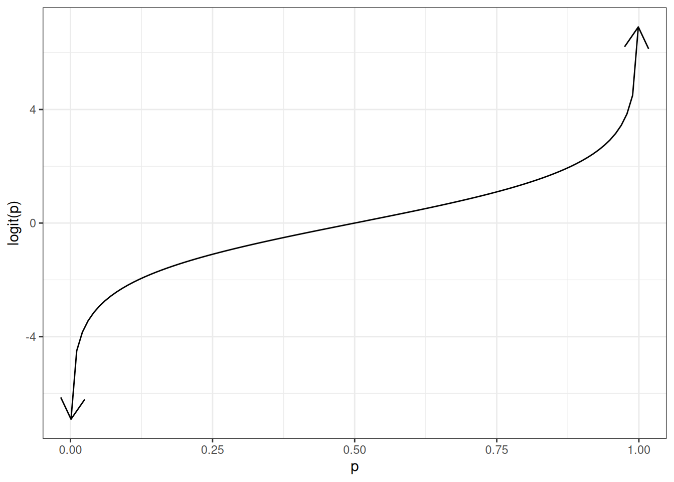
Theorem 10 If \(\pi\) is the probability of an event \(A\), \(\omega\) is the corresponding odds of \(A\), and \(\eta\) is the corresponding log-odds of \(A\), then:

\[\eta= \text{log}{\left\{\frac{\pi}{1-\pi}\right\}} \tag{12}\]

Proof. Apply Definition 13 and then Theorem 2.

Definition 14 (logit function)  

The logit function of a probability \(\pi\) is the natural logarithm of the odds function of \(\pi\):

\[\text{logit}(\pi) \stackrel{\text{def}}{=}\text{log}{\left\{\text{odds}{\left\{\pi\right\}}\right\}}\]

The logit function is a composite function.

Exercise 25 (Compose the logit function) Mathematically expand the definition of the logit function.

Solution 19 (Compose the logit function).

Theorem 11 (Expanded expression for logit) \[\text{logit}(\pi) = \text{log}{\left\{\frac{\pi}{1-\pi}\right\}} \tag{13}\]

Proof. Apply Definition 14 and then Definition 8 (details left to the reader).

Corollary 6 If \(\pi\) is the probability of an event \(A\) and \(\eta\) is the corresponding log-odds of \(A\), then:

\[\eta= \text{logit}{\left\{\pi\right\}}\]

Proof. Apply Theorem 10 and Theorem 11.

Figure 4 shows the shape of the \(\text{logit}()\) function.

odds <- function(pi) pi / (1 - pi)

logit <- function(p) log(odds(p))

library(ggplot2)
logit_plot <-
  ggplot() +
  geom_function(
    fun = logit,
    arrow = arrow(ends = "both")
  ) +
  xlim(.001, .999) +
  ylab("logit(p)") +
  xlab("p") +
  theme_bw()
print(logit_plot)

Figure 4: The logit function

The expit function

Lemma 3  

If \(\omega\) is the odds of an event \(A\) and \(\eta\) is the corresponding log-odds of \(A\), then:

\[\omega= \text{exp}{\left\{\eta\right\}}\]

Proof. Start from Definition 13 and solve for \(\omega\).

Theorem 12  

If \(\pi\) is the probability of an event \(A\), \(\omega\) is the corresponding odds of \(A\), and \(\eta\) is the corresponding log-odds of \(A\), then:

\[\pi= \frac{\text{exp}{\left\{\eta\right\}}}{1+\text{exp}{\left\{\eta\right\}}}\]

Proof. Apply Theorem 6 and then Lemma 3.

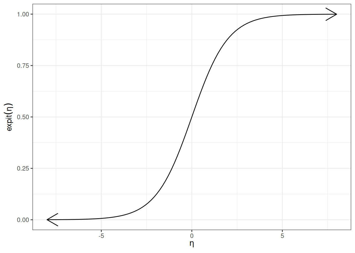
Definition 15 (expit, logistic, inverse-logit) The expit function of a log-odds \(\eta\), also known as the inverse-logit function or logistic function, is the inverse-odds of the exponential of \(\eta\):

\[\text{expit}(\eta) \stackrel{\text{def}}{=}\text{invodds}{\left\{\text{exp}{\left\{\eta\right\}}\right\}}\]

Theorem 13 (Expressions for expit function) \[ \begin{aligned} \text{expit}(\eta) &= \frac{\text{exp}{\left\{\eta\right\}}}{1+\text{exp}{\left\{\eta\right\}}} \\ &= \frac{1}{1 + \text{exp}{\left\{-\eta\right\}})} \\ &= (1 + \text{exp}{\left\{-\eta\right\}})^{-1} \end{aligned} \]

Proof. Apply definitions and Lemma 1. Details left to the reader.

Theorem 14 If \(\pi\) is the probability of an event \(A\), \(\omega\) is the corresponding odds of \(A\), and \(\eta\) is the corresponding log-odds of \(A\), then:

\[\pi= \text{expit}{\left\{\eta\right\}}\]

Proof. Apply Theorem 12 and Theorem 13.

Figure 5 graphs the expit function.

expit <- function(eta) {
  exp(eta) / (1 + exp(eta))
}
library(ggplot2)
expit_plot <-
  ggplot() +
  geom_function(
    fun = expit,
    arrow = arrow(ends = "both")
  ) +
  xlim(-8, 8) +
  ylim(0, 1) +
  ylab(expression(expit(eta))) +
  xlab(expression(eta)) +
  theme_bw()
print(expit_plot)

Figure 5: The expit function

Theorem 15 (logit and expit are each others’ inverses) \[\text{logit}{\left\{\text{expit}{\left\{\eta\right\}}\right\}} = \eta\]

\[\text{expit}{\left\{\text{logit}{\left\{\pi\right\}}\right\}} = \pi\]

Proof. Left to the reader.

Diagram of expit and logit

Figure 6: Diagram of logistic regression link and inverse link functions

\[ \underbrace{\pi}_{\atop{\Pr(Y=1)} } \overbrace{ \underbrace{ \underset{ \xleftarrow[\frac{\omega}{1+\omega}]{} } { \xrightarrow{\frac{\pi}{1-\pi}} } \underbrace{\omega}_{\text{odds}(Y=1)} \underset{ \xleftarrow[\text{exp}{\left\{\eta\right\}}]{} } { \xrightarrow{\text{log}{\left\{\omega\right\}}} } }_{\text{expit}(\eta)} }^{\text{logit}(\pi)} \underbrace{\eta}_{\atop{\text{log-odds}(Y=1)}} \]

2 Introduction to logistic regression

• In Example 1, we estimated the risk and the odds of MI for two groups, defined by oral contraceptive use.

• If the predictor is quantitative (dose) or there is more than one predictor, the task becomes more difficult.

• In this case, we will use logistic regression, which is a generalization of the linear regression models you have been using that can account for a binary response instead of a continuous one.

Independent binary outcomes - general

Exercise 26 Let \(\tilde{y}\) represent a data set of mutually independent binary outcomes, each with a potentially different event probability \(\pi_i\):

\[ \begin{aligned} \tilde{y}&= (y_1, ..., y_n) \\ y_i &\ \sim_{\perp\!\!\!\perp}\ \text{Ber}(\pi_i) \end{aligned} \]

Write the likelihood of \(\tilde{y}\).

Solution 20. \[ \begin{aligned} {\color{red}\pi_i} &\stackrel{\text{def}}{=}\text{P}(Y_i=1) \\ \text{P}(Y_i=0) &= 1-{\color{red}\pi_i} \\ \text{P}(Y_i=y_i) &= \text{P}(Y_i=1)^{y_i} \text{P}(Y_i=0)^{1-y_i} \\ &= (\pi_i)^{y_i} (1-\pi_i)^{1-y_i} \\ {\color{red}\mathscr{L}_i(\pi_i)} &\stackrel{\text{def}}{=}\text{P}(Y_i=y_i) \\ \mathscr{L}(\tilde{\pi}) &\stackrel{\text{def}}{=}\text{P}(Y_1=y_1, \ldots, Y_n = y_n) \\ &= \prod_{i=1}^n\text{P}(Y_i=y_i) \\ &= \prod_{i=1}^n{\color{red}\mathscr{L}_i(\pi_i)} \\ &= \prod_{i=1}^n(\pi_i)^{y_i} (1-\pi_i)^{1-y_i} \end{aligned} \]

Exercise 27 Write the log-likelihood of \(\tilde{y}\).

Solution 21. \[ \begin{aligned} \ell(\tilde{\pi}) &\stackrel{\text{def}}{=}\text{log}{\left\{\mathscr{L}(\tilde{\pi})\right\}} \\ &= \text{log}{\left\{\prod_{i=1}^n\mathscr{L}_i(\pi_i)\right\}} \\ &= \sum_{i=1}^n\text{log}{\left\{\mathscr{L}_i(\pi_i)\right\}} \\ &= \sum_{i=1}^n\ell_i(\pi_i) \\ \ell_i(\pi_i) &\stackrel{\text{def}}{=}\text{log}{\left\{\mathscr{L}_i(\pi_i)\right\}} \\ &= y_i \text{log}{\left\{\pi_i\right\}} + (1-y_i) \text{log}{\left\{1-\pi_i\right\}} \end{aligned} \]

Modeling \(\pi_i\) as a function of \(X_i\)

If there are only a few distinct \(X_i\) values, we can model \(\pi_i\) separately for each value of \(X_i\).

Otherwise, we need regression.

\[ \begin{aligned} \pi(x) &\equiv \text{E}(Y=1|X=x)\\ &= f(x^\top\beta) \end{aligned} \]

Typically, we use the \(\text{expit}\) inverse-link:

\[\pi(\tilde{x}) = \text{expit}(\tilde{x}'\beta) \tag{14}\]

Meet the beetles

library(glmx)
library(dplyr)
data(BeetleMortality, package = "glmx")
beetles <- BeetleMortality |>
  mutate(
    pct = died / n,
    survived = n - died,
    dose_c = dose - mean(dose)
  )
beetles

Table 4: Mortality rates of adult flour beetles after five hours’ exposure to gaseous carbon disulphide (Bliss 1935)

library(ggplot2)
plot1 <-
  beetles |>
  ggplot(aes(x = dose, y = pct)) +
  geom_point(aes(size = n)) +
  xlab("Dose (log mg/L)") +
  ylab("Mortality rate (%)") +
  scale_y_continuous(labels = scales::percent) +
  scale_size(range = c(1, 2)) +
  theme_bw(base_size = 18)

print(plot1)

Figure 7: Mortality rates of adult flour beetles after five hours’ exposure to gaseous carbon disulphide (Bliss 1935)

Why don’t we use linear regression?

beetles_long <- beetles |>
  reframe(
    .by = everything(),
    outcome = c(
      rep(1, times = died),
      rep(0, times = survived)
    )
  ) |>
  as_tibble()

lm1 <- beetles_long |> lm(formula = outcome ~ dose)
f_linear <- function(x) predict(lm1, newdata = data.frame(dose = x))

range1 <- range(beetles$dose) + c(-.2, .2)

plot2 <-
  plot1 +
  geom_function(
    fun = f_linear,
    aes(col = "Straight line")
  ) +
  labs(colour = "Model", size = "")

plot2 |> print()

Figure 8: Mortality rates of adult flour beetles after five hours’ exposure to gaseous carbon disulphide (Bliss 1935)

Zoom out

(plot2 + expand_limits(x = c(1.6, 2))) |> print()

Figure 9: Mortality rates of adult flour beetles after five hours’ exposure to gaseous carbon disulphide (Bliss 1935)

log transformation of dose?

lm2 <- beetles_long |> lm(formula = outcome ~ log(dose))
f_linearlog <- function(x) predict(lm2, newdata = data.frame(dose = x))

plot3 <- plot2 +
  expand_limits(x = c(1.6, 2)) +
  geom_function(fun = f_linearlog, aes(col = "Log-transform dose"))
(plot3 + expand_limits(x = c(1.6, 2))) |> print()

Figure 10: Mortality rates of adult flour beetles after five hours’ exposure to gaseous carbon disulphide (Bliss 1935)

Logistic regression

beetles_glm_grouped <- beetles |>
  glm(formula = cbind(died, survived) ~ dose, family = "binomial")
f <- function(x) {
  beetles_glm_grouped |>
    predict(newdata = data.frame(dose = x), type = "response")
}

plot4 <- plot3 + geom_function(fun = f, aes(col = "Logistic regression"))
plot4 |> print()

Figure 11: Mortality rates of adult flour beetles after five hours’ exposure to gaseous carbon disulphide (Bliss 1935).

Three parts to regression models

• What distribution does the outcome have for a specific subpopulation defined by covariates? (outcome model)

• How does the combination of covariates relate to the mean? (link function)

• How do the covariates combine? (linear predictor, interactions)

Fitting and manipulating logistic regression models in R

library(glmx)
library(dplyr)
data(BeetleMortality)
beetles <- BeetleMortality |>
  mutate(
    pct = died / n,
    survived = n - died
  )

beetles_glm_grouped <-
  beetles |>
  glm(
    formula = cbind(died, survived) ~ dose,
    family = "binomial"
  )

library(parameters)
beetles_glm_grouped |>
  parameters() |>
  print_md()

Table 5: logistic regression model for beetles data with grouped (binomial) data

Parameter	Log-Odds	SE	95% CI	z	p
(Intercept)	-60.72	5.18	(-71.44, -51.08)	-11.72	< .001
dose	34.27	2.91	(28.85, 40.30)	11.77	< .001

Fitted values

Fitted values are provided on the probability scale (Table 6)

Table 6

fitted(beetles_glm_grouped)
#>        1        2        3        4        5        6        7        8 
#> 0.058601 0.164028 0.362119 0.605315 0.795172 0.903236 0.955196 0.979049
predict(beetles_glm_grouped, type = "response")
#>        1        2        3        4        5        6        7        8 
#> 0.058601 0.164028 0.362119 0.605315 0.795172 0.903236 0.955196 0.979049

Count scale

For grouped data, we can convert to the count scale by multiplying by the group size:

beetles$n * fitted(beetles_glm_grouped)
#>        1        2        3        4        5        6        7        8 
#>  3.45746  9.84167 22.45138 33.89763 50.09582 53.29091 59.22216 58.74296

Logit scale

predict(beetles_glm_grouped, type = "link")
#>         1         2         3         4         5         6         7         8 
#> -2.776615 -1.628559 -0.566179  0.427661  1.356386  2.233707  3.059622  3.844412

Converting between logit and probability scales works as expected:

predict(beetles_glm_grouped, type = "link") |> arm::invlogit()
#>        1        2        3        4        5        6        7        8 
#> 0.058601 0.164028 0.362119 0.605315 0.795172 0.903236 0.955196 0.979049
predict(beetles_glm_grouped, type = "response")
#>        1        2        3        4        5        6        7        8 
#> 0.058601 0.164028 0.362119 0.605315 0.795172 0.903236 0.955196 0.979049

predict(beetles_glm_grouped, type = "response") |> arm::logit()
#>         1         2         3         4         5         6         7         8 
#> -2.776615 -1.628559 -0.566179  0.427661  1.356386  2.233707  3.059622  3.844412
predict(beetles_glm_grouped, type = "link")
#>         1         2         3         4         5         6         7         8 
#> -2.776615 -1.628559 -0.566179  0.427661  1.356386  2.233707  3.059622  3.844412

type = "terms" is confusing, because the variables get centered:

predict(beetles_glm_grouped, type = "terms")
#>        dose
#> 1 -3.520419
#> 2 -2.372363
#> 3 -1.309983
#> 4 -0.316144
#> 5  0.612582
#> 6  1.489902
#> 7  2.315817
#> 8  3.100608
#> attr(,"constant")
#> [1] 0.743804
coef(beetles_glm_grouped)["dose"] * beetles$dose
#> [1] 57.9408 59.0889 60.1513 61.1451 62.0738 62.9512 63.7771 64.5619

We can construct the link-scale predictions from the terms:

terms_pred <- predict(beetles_glm_grouped, type = "terms")
terms_pred + attr(terms_pred, "constant")
#>        dose
#> 1 -2.776615
#> 2 -1.628559
#> 3 -0.566179
#> 4  0.427661
#> 5  1.356386
#> 6  2.233707
#> 7  3.059622
#> 8  3.844412
#> attr(,"constant")
#> [1] 0.743804
predict(beetles_glm_grouped, type = "link")
#>         1         2         3         4         5         6         7         8 
#> -2.776615 -1.628559 -0.566179  0.427661  1.356386  2.233707  3.059622  3.844412

Individual observations

beetles_long

Table 7: beetles data in long format

beetles_glm_ungrouped <-
  beetles_long |>
  glm(
    formula = outcome ~ dose,
    family = "binomial"
  )

beetles_glm_ungrouped |>
  parameters() |>
  print_md()

Table 8: logistic regression model for beetles data with individual Bernoulli data

Parameter	Log-Odds	SE	95% CI	z	p
(Intercept)	-60.72	5.18	(-71.44, -51.08)	-11.72	< .001
dose	34.27	2.91	(28.85, 40.30)	11.77	< .001

Exercise 28 Compare this model with the grouped-observations model (Table 5).

Solution 22.

They seem the same! But not quite:

logLik(beetles_glm_grouped)
#> 'log Lik.' -18.7151 (df=2)
logLik(beetles_glm_ungrouped)
#> 'log Lik.' -186.235 (df=2)

The difference is due to the binomial coefficient \(\left(n\atop x \right)\) which isn’t included in the individual-observations (Bernoulli) version of the model.

3 Derivatives of logistic regression functions

In order to interpret logistic regression models and find their MLEs, we will need to compute various derivatives. This section compiles some useful results.

Derivatives of odds function

Theorem 16 (Derivative of odds function) \[{\text{odds}}'{\left\{\pi\right\}} = \frac{\partial \omega}{\partial \pi} = \frac{1}{{\left(1-\pi\right)}^2}\]

Proof. We can use Theorem 2 and the quotient rule:

\[ \begin{aligned} \frac{\partial \omega}{\partial \pi} &= \frac{\partial}{\partial \pi}{\left(\frac{\pi}{1-\pi}\right)} \\ &= \frac {\frac{\partial}{\partial \pi}\pi} {1-\pi} - {\left(\frac{\pi}{{\left(1-\pi\right)}^2} \cdot\frac{\partial}{\partial \pi}{\left(1-\pi\right)}\right)} \\ &= \frac{1}{1-\pi} - \frac{\pi}{{\left(1-\pi\right)}^2} \cdot(-1) \\ &= \frac{1}{1-\pi} + \frac{\pi}{{\left(1-\pi\right)}^2} \\ &= \frac{1-\pi}{{\left(1-\pi\right)}^2} + \frac{\pi}{{\left(1-\pi\right)}^2} \\ &= \frac{1-\pi + \pi}{{\left(1-\pi\right)}^2} \\ &= \frac{1}{{\left(1-\pi\right)}^2} \end{aligned} \]

Corollary 7 \[\frac{\partial \omega}{\partial \pi} = {\left(1+\omega\right)}^2\]

Proof. By Theorem 16 and Corollary 5.

Derivatives of inverse-odds function

Theorem 17 (Derivative of inverse odds function) \[{\text{invodds}}'{\left\{\omega\right\}} = \frac{\partial \pi}{\partial \omega} = (1-\pi)^2 = \frac{1}{{\left(1+\omega\right)}^2} \tag{15}\]

Proof. By Theorem 16 and Corollary 7.

Or for a direct approach, use the quotient rule again:

\[ \begin{aligned} \frac{\partial \pi}{\partial \omega} &= \frac{\partial}{\partial \omega} \frac{\omega}{1+\omega} \\ &= \frac{\frac{\partial}{\partial \omega}\omega}{1+\omega} - \frac{\omega}{{\left(1+\omega\right)}^2} \cdot\frac{\partial}{\partial \omega}(1+\omega) \\ &= \frac{1}{1+\omega} - \frac{\omega}{{\left(1+\omega\right)}^2} \cdot 1 \\ &= \frac{1}{1+\omega} - \frac{\omega}{{\left(1+\omega\right)}^2} \\ &= \frac{1+\omega}{{\left(1+\omega\right)}^2} - \frac{\omega}{{\left(1+\omega\right)}^2} \\ &= \frac{1+\omega- \omega}{{\left(1+\omega\right)}^2} \\ &= \frac{1}{{\left(1+\omega\right)}^2} \end{aligned} \]

Derivatives of logit function

Lemma 4 (Derivative of log-odds by odds) \[\frac{\partial \eta}{\partial \omega} = \omega^{-1}\]

Proof. Using Definition 13:

\[ \begin{aligned} \frac{\partial \eta}{\partial \omega} &= \frac{\partial}{\partial \omega}\log{\omega} \\ &= \omega^{-1} \end{aligned} \]

Theorem 18 (Derivative of log-odds by odds) \[\frac{\partial \eta}{\partial \omega} = \frac{1-\pi}{\pi}\]

Proof. Using Theorem 2 and Lemma 4:

\[ \begin{aligned} \frac{\partial \eta}{\partial \omega} &= \omega^{-1} \\ &= \frac{1-\pi}{\pi} \end{aligned} \]

Theorem 19 (Derivative of log-odds by probability) \[\frac{\partial \eta}{\partial \pi} = \frac{1}{(\pi)(1-\pi)}\]

Proof. Using Theorem 18, Theorem 16, and the chain rule:

\[ \begin{aligned} \frac{\partial \eta}{\partial \pi} &= \frac{\partial \eta}{\partial \omega} \frac{\partial \omega}{\partial \pi} \\ &= \frac{1-\pi}{\pi} \frac{1}{{\left(1-\pi\right)}^2} \\ &= \frac{1}{(\pi)(1-\pi)} \end{aligned} \]

Corollary 8 (Derivative of logit function) \[\text{logit}'(\pi) = \frac{1}{(\pi)(1-\pi)}\]

Proof. By Theorem 19 and Corollary 6.

Derivatives of expit function

Lemma 5 \[\frac{\partial \omega}{\partial \eta} = \omega\]

Proof. Using Lemma 3 and the derivative of the exponential function:

\[ \begin{aligned} \frac{\partial \omega}{\partial \eta} &= \frac{\partial}{\partial \eta} \text{exp}{\left\{\eta\right\}} \\ &= \text{exp}{\left\{\eta\right\}} \\ &= \omega \end{aligned} \]

Theorem 20 \[\frac{\partial \omega}{\partial \eta} = \frac{\pi}{1-\pi} \tag{16}\]

Proof. Use Lemma 5 and Theorem 2.

Theorem 21 \[\frac{\partial \pi}{\partial \eta} = \pi (1-\pi)\]

Proof. By the chain rule, Theorem 20, and Theorem 17:

\[ \begin{aligned} \frac{\partial \pi}{\partial \eta} &= {\color{green}\frac{\partial \omega}{\partial \eta}}{\color{blue}\frac{\partial \pi}{\partial \omega}} \\ &= {\color{green}\frac{\pi}{1-\pi}} {\color{blue}(1-\pi)^2} \\ &= \pi (1-\pi) \end{aligned} \]

Alternatively, by Theorem 19:

\[ \begin{aligned} \frac{\partial \pi}{\partial \eta} &= {\left(\frac{\partial \eta}{\partial \pi}\right)}^{-1} \\ &= {\left(\frac{1}{(\pi)(1-\pi)}\right)}^{-1} \\ &= \pi (1-\pi) \end{aligned} \]

Corollary 9 If \(\pi = \Pr(Y=1| \tilde{X}=\tilde{x})\), then:

\[\frac{\partial \pi}{\partial \eta} = \text{Var}{\left(Y|X=x\right)}\]

4 Understanding logistic regression models

Lemma 6 By the derivative of a linear combination:

\[ \begin{aligned} \frac{\partial \eta}{\partial \tilde{x}} &= \frac{\partial}{\partial \tilde{x}} \tilde{x}\cdot \tilde{\beta} \\ &= \tilde{\beta} \end{aligned} \]

Exercise 29 Consider a logistic regression model with a single predictor, \(X\):

\[ \begin{aligned} Y_i|X_i &\ \sim_{\perp\!\!\!\perp}\ \text{Ber}(\pi(X_i)) \\ \pi(x) &= \text{expit}{\left\{\eta(x)\right\}} = \pi(\omega(\eta(x))) \\ \eta(x) &= \alpha + \beta x \end{aligned} \tag{17}\]

Find the derivative of \(\pi(x) = \text{E}{\left[Y|X=x\right]}\) with respect to \(x\):

\[\frac{\partial \pi}{\partial x} = ?\]

Solution 23. By Theorem 21, Lemma 6, and the chain rule:

\[ \begin{aligned} \frac{\partial \pi}{\partial x} &={\color{red}\frac{\partial \pi}{\partial \eta}} {\color{blue}\frac{\partial \eta}{\partial x}} \\ &= {\color{red}\pi (1-\pi)} {\color{blue}\beta} \\ &= {\color{red}\text{Var}{\left(Y|X=x\right)}} \cdot {\color{blue}\beta} \end{aligned} \]

The slope is steepest at \(\pi = 0.5\), i.e., at \(\eta = 0\), which for a unipredictor model occurs at \(x = -\alpha/\beta\). The slope goes to 0 as \(x\) goes to \(-\infty\) or \(+\infty\) (compare with Figure 5).

Note

In order to interpret \(\beta_j\): differentiate or difference \({\color{red}\eta(\tilde{x})}\) with respect to \({\color{red}x_j}\) (depending on whether \(x_j\) is continuous or discrete, respectively):

\[\frac{\partial}{\partial {\color{red}x_j}} {\color{red}\eta(\tilde{x})}\]

In order to find the MLE \(\hat{\tilde{\beta}}\): differentiate the log-likelihood function \({\color{blue}\ell(\tilde{\beta})}\) with respect to \({\color{blue}\tilde{\beta}}\):

\[\frac{\partial}{\partial {\color{blue}\tilde{\beta}}} {\color{blue}\ell(\tilde{\beta})}\]

Exercise 30 (General formula for odds ratios in logistic regression) Consider the generic logistic regression model:

• \(Y_i|\tilde{X}_i \ \sim_{\perp\!\!\!\perp}\ \text{Ber}(\pi(\tilde{X}_i))\)
• \(\text{logit}{\left\{\pi(\tilde{x})\right\}} = \eta(\tilde{x})\)
• \(\eta(\tilde{x}) = \tilde{x}'\tilde{\beta}\)

Let \(\tilde{x}\) and \({\tilde{x}^*}\) be two covariate patterns, representing two individuals or two subpopulations.

Find a concise formula to compute the odds ratio comparing covariate patterns \(\tilde{x}\) and \({\tilde{x}^*}\):

\[\theta(\tilde{x},{\tilde{x}^*}) \stackrel{\text{def}}{=}\frac{\omega(\tilde{x})}{\omega({\tilde{x}^*})} \tag{18}\]

Solution 24 (General formula for odds ratios in logistic regression). \[ \begin{aligned} \theta(\tilde{x},{\tilde{x}^*}) &\stackrel{\text{def}}{=}\frac{\omega(\tilde{x})}{\omega({\tilde{x}^*})} \\ &= \frac{\text{exp}{\left\{\eta(\tilde{x})\right\}}}{\text{exp}{\left\{\eta({\tilde{x}^*})\right\}}} \\ &= \text{exp}{\left\{{\color{red}\eta(\tilde{x}) - \eta({\tilde{x}^*})}\right\}} \end{aligned} \]

Solution 24 is more concrete than Equation 18, but it doesn’t yet completely explain how to compute \(\theta(\tilde{x},{\tilde{x}^*})\), so let’s mark it as a lemma:

Lemma 7 (General formula for odds ratios in logistic regression) \[\theta(\tilde{x},{\tilde{x}^*}) = \text{exp}{\left\{{\color{red}\eta(\tilde{x}) - \eta({\tilde{x}^*})}\right\}} \tag{19}\]

Proof. By Solution 24.

Definition 16 (Difference in log-odds)  

Let \(\tilde{x}\) and \({\tilde{x}^*}\) be two covariate patterns, representing two individuals or two subpopulations.

Then we can define the difference in log-odds between \(\tilde{x}\) and \({\tilde{x}^*}\), denoted \(\Delta \eta(\tilde{x}, {\tilde{x}^*})\) or \(\Delta \eta\) for short, as:

\[{\color{red}\Delta \eta} \stackrel{\text{def}}{=}{\color{red}\eta(\tilde{x}) - \eta({\tilde{x}^*})}\]

Corollary 10 (Shorthand general formula for odds ratios in logistic regression) \[\theta(\tilde{x},{\tilde{x}^*}) = \text{exp}{\left\{{\color{red}\Delta \eta}\right\}} \tag{20}\]

Proof. By Lemma 7 and Definition 16.

Exercise 31 (Difference in log-odds) Find a concise expression for the difference in log-odds: \[\Delta \eta\stackrel{\text{def}}{=}{\color{red}\eta(\tilde{x}) - \eta({\tilde{x}^*})}\]

Solution 25 (Difference in log-odds). \[ \begin{aligned} {\color{red}\Delta \eta} &\stackrel{\text{def}}{=}{\color{red}\eta(\tilde{x}) - \eta({\tilde{x}^*})} \\ &= (\tilde{x}\cdot\tilde{\beta}) - ({\tilde{x}^*}\cdot\tilde{\beta}) \\ &= (\tilde{x}^{\top}\tilde{\beta}) - ({\left({\tilde{x}^*}\right)}^{\top}\tilde{\beta}) \\ &= (\tilde{x}^{\top} - {\left({\tilde{x}^*}\right)}^{\top})\tilde{\beta} \\ &= (\tilde{x}- {\tilde{x}^*})^{\top}\tilde{\beta} \\ &= ({\color{blue}\tilde{x}- {\tilde{x}^*}})\cdot\tilde{\beta} \end{aligned} \]

Lemma 8 (Difference in log-odds) \[{\color{red}\Delta \eta}= ({\color{blue}\tilde{x}- {\tilde{x}^*}})\cdot\tilde{\beta}\]

Proof. By Solution 25.

Definition 17 (Difference in covariate patterns)  

Let \(\tilde{x}\) and \({\tilde{x}^*}\) be two covariate patterns, representing two individuals or two subpopulations. The difference in covariate patterns, denoted \(\Delta\tilde{x}\), is defined as:

\[{\color{blue}\Delta\tilde{x}} \stackrel{\text{def}}{=}{\color{blue}\tilde{x}- {\tilde{x}^*}}\]

Corollary 11 (Difference in log-odds) \[{\color{red}\Delta \eta}= ({\color{blue}\Delta\tilde{x}}) \cdot \tilde{\beta}\]

Proof. By Lemma 8 and Definition 17.

Exercise 32 Find an expression for the odds ratio \(\theta(\tilde{x},{\tilde{x}^*})\) in terms of \(\Delta\tilde{x}\) and \(\tilde{\beta}\).

Solution 26. Combine Corollary 10 and Corollary 11:

\[ \begin{aligned} \theta(\tilde{x},{\tilde{x}^*}) &= \text{exp}{\left\{\Delta \eta\right\}} \\ &= \text{exp}{\left\{\Delta\tilde{x}\cdot \tilde{\beta}\right\}} \end{aligned} \]

Theorem 22 The odds ratio comparing covariate patterns \(\tilde{x}\) and \({\tilde{x}^*}\) is:

\[\theta(\tilde{x},{\tilde{x}^*}) = \text{exp}{\left\{(\Delta\tilde{x}) \cdot \tilde{\beta}\right\}} \tag{21}\]

Proof. By Solution 26.

Corollary 12 \[\text{log}{\left\{\theta(\tilde{x},{\tilde{x}^*})\right\}} = \Delta \eta\]

5 Estimating logistic regression models

Model

Assume:

• \(Y_i|\tilde{X}_i \ \sim_{\perp\!\!\!\perp}\ \text{Ber}(\pi(X_i))\)
• \(\pi(\tilde{x}) = \text{expit}{\left\{\eta(\tilde{x})\right\}}\)
• \(\eta(\tilde{x}) = \tilde{x}\cdot \tilde{\beta}\)

Likelihood function

Exercise 33 Compute and graph the likelihood for the beetles data model:

library(glmx)
library(dplyr)
data(BeetleMortality)
beetles <- BeetleMortality |>
  mutate(
    pct = died / n,
    survived = n - died,
    dose_c = dose - mean(dose)
  )
beetles_long <-
  beetles |>
  reframe(
    .by = everything(),
    outcome = c(
      rep(1, times = died),
      rep(0, times = survived)
    )
  )
beetles

Table 9: Mortality rates of adult flour beetles after five hours’ exposure to gaseous carbon disulphide (Bliss 1935)

beetles_glm <-
  beetles |>
  glm(
    formula = cbind(died, survived) ~ dose,
    family = "binomial"
  )
equatiomatic::extract_eq(beetles_glm)

\[ \log\left[ \frac { P( \operatorname{died} = \operatorname{60} ) }{ 1 - P( \operatorname{died} = \operatorname{60} ) } \right] = \alpha + \beta_{1}(\operatorname{dose}) \]

beetles_glm |> 
  parameters::parameters() |> 
  parameters::print_md()

Table 10: Fitted logistic regression model for beetles data

Parameter	Log-Odds	SE	95% CI	z	p
(Intercept)	-60.72	5.18	(-71.44, -51.08)	-11.72	< .001
dose	34.27	2.91	(28.85, 40.30)	11.77	< .001

Solution 27.

odds_inv <- function(omega) (1 + omega^-1)^-1
lik_beetles0 <- function(beta_0, beta_1) {
  beetles |>
    mutate(
      eta = beta_0 + beta_1 * dose,
      omega = exp(eta),
      pi = odds_inv(omega),
      Lik = pi^died * (1 - pi)^survived,
      # llik = died*eta + n*log(1 - pi)
    ) |>
    pull(Lik) |>
    prod()
}

lik_beetles <- Vectorize(lik_beetles0)

ranges <- beetles_glm |> confint.default(level = 0.05)

n_points <- 25
beta_0s <- seq(
  ranges["(Intercept)", 1],
  ranges["(Intercept)", 2],
  length.out = n_points
)
beta_1s <- seq(
  ranges["dose", 1],
  ranges["dose", 2],
  length.out = n_points
)
names(beta_0s) <- round(beta_0s, 2)
names(beta_1s) <- round(beta_1s, 2)

if (run_graphs) {
  lik_mat_beetles <- outer(beta_0s, beta_1s, lik_beetles)
  plotly::plot_ly(
    type = "surface",
    x = ~beta_0s,
    y = ~beta_1s,
    z = ~ t(lik_mat_beetles)
  )
  # see https://stackoverflow.com/questions/69472185/correct-use-of-coordinates-to-plot-surface-data-with-plotly 
  # for explanation of why transpose `t()` is needed
  
}

Figure 12: Likelihood of beetles data. Bumps on ridge are artifacts of render; increase n_points to improve render quality.

Log-likelihood function

Exercise 34 Find the log-likelihood function for the general logistic regression model.

Solution 28. \[ \begin{aligned} \ell(\tilde{\beta}, \tilde{y}) &= \text{log}{\left\{\mathscr{L}(\tilde{\beta}, \tilde{y}) \right\}} \\ &= \sum_{i=1}^n{\color{red}\ell_i}(\pi(\tilde{x}_i)) \end{aligned} \tag{22}\]

Using Theorem 10 and Corollary 5: \[ \begin{aligned} {\color{red}\ell_i}(\pi_i) &= y_i \text{log}{\left\{\pi_i\right\}} + (1 - y_i) \text{log}{\left\{1-\pi_i\right\}} \\ &= y_i \text{log}{\left\{\pi_i\right\}} + (1 \cdot\text{log}{\left\{1-\pi_i\right\}} - y_i \cdot\text{log}{\left\{1-\pi_i\right\}}) \\ &= y_i \text{log}{\left\{\pi_i\right\}} + (\text{log}{\left\{1-\pi_i\right\}} - y_i \text{log}{\left\{1-\pi_i\right\}}) \\ &= y_i \text{log}{\left\{\pi_i\right\}} + \text{log}{\left\{1-\pi_i\right\}} - y_i \text{log}{\left\{{\color{blue}1-\pi_i}\right\}} \\ &= y_i \text{log}{\left\{\pi_i\right\}} - y_i \text{log}{\left\{{\color{blue}1-\pi_i}\right\}} + \text{log}{\left\{1-\pi_i\right\}} \\ &= (y_i \text{log}{\left\{\pi_i\right\}} - y_i \text{log}{\left\{{\color{blue}1-\pi_i}\right\}}) + \text{log}{\left\{1-\pi_i\right\}} \\ &= y_i (\text{log}{\left\{{\color{red}\pi_i}\right\}} - \text{log}{\left\{{\color{blue}1-\pi_i}\right\}}) + \text{log}{\left\{1-\pi_i\right\}} \\ &= y_i {\left(\text{log}{\left\{\frac{{\color{red}\pi_i}}{{\color{blue}1-\pi_i}}\right\}}\right)} + \text{log}{\left\{1-\pi_i\right\}} \\ &= y_i \text{logit}(\pi_i) + \text{log}{\left\{1-\pi_i\right\}} \\ &= y_i \eta_i + \text{log}{\left\{1-\pi_i\right\}} \\ &= y_i \eta_i + \text{log}{\left\{{\left(1+\omega_i\right)}^{-1}\right\}} \\ &= y_i \eta_i - \text{log}{\left\{1+\omega_i\right\}} \end{aligned} \]

Lemma 9 \[\ell_i(\pi_i) = y_i \eta_i - \text{log}{\left\{1+\omega_i\right\}}\]

Exercise 35 Compute and graph the log-likelihood for the beetles data.

Solution 29.

odds_inv <- function(omega) (1 + omega^-1)^-1
llik_beetles0 <- function(beta_0, beta_1) {
  beetles |>
    mutate(
      eta = beta_0 + beta_1 * dose,
      omega = exp(eta),
      pi = odds_inv(omega), # need for next line:
      llik = died*eta + n*log(1 - pi)
    ) |>
    pull(llik) |>
    sum()
}

llik_beetles <- Vectorize(llik_beetles0)

# to check that we implemented it correctly:
# ests = coef(beetles_glm_ungrouped)
# logLik(beetles_glm_ungrouped)
# llik_beetles(ests[1], ests[2])

if (run_graphs) {
  llik_mat_beetles <- outer(beta_0s, beta_1s, llik_beetles)
  plotly::plot_ly(
    type = "surface",
    x = ~beta_0s,
    y = ~beta_1s,
    z = ~ t(llik_mat_beetles)
  )
}

Figure 13: log-likelihood of beetles data

Let’s center dose:

beetles_glm_grouped_centered <- beetles |>
  glm(
    formula = cbind(died, survived) ~ dose_c,
    family = "binomial"
  )

beetles_glm_ungrouped_centered <- beetles_long |>
  mutate(died = outcome) |>
  glm(
    formula = died ~ dose_c,
    family = "binomial"
  )

equatiomatic::extract_eq(beetles_glm_ungrouped_centered)

\[ \log\left[ \frac { P( \operatorname{died} = \operatorname{1} ) }{ 1 - P( \operatorname{died} = \operatorname{1} ) } \right] = \alpha + \beta_{1}(\operatorname{dose\_c}) \]

beetles_glm_grouped_centered |> 
  parameters::parameters() |> 
  parameters::print_md()

Table 11: Fitted logistic regression model for beetles data, with dose centered

Parameter	Log-Odds	SE	95% CI	z	p
(Intercept)	0.74	0.14	(0.48, 1.02)	5.40	< .001
dose c	34.27	2.91	(28.85, 40.30)	11.77	< .001

odds_inv <- function(omega) (1 + omega^-1)^-1
lik_beetles0 <- function(beta_0, beta_1) {
  beetles |>
    mutate(
      eta = beta_0 + beta_1 * dose_c,
      omega = exp(eta),
      pi = odds_inv(omega),
      Lik = (pi^died) * (1 - pi)^(survived)
    ) |>
    pull(Lik) |>
    prod()
}

lik_beetles <- Vectorize(lik_beetles0)

ranges <- beetles_glm_grouped_centered |> confint.default(level = .95)

n_points <- 25
beta_0s <- seq(
  ranges["(Intercept)", 1],
  ranges["(Intercept)", 2],
  length.out = n_points
)
beta_1s <- seq(
  ranges["dose_c", 1],
  ranges["dose_c", 2],
  length.out = n_points
)
names(beta_0s) <- round(beta_0s, 2)
names(beta_1s) <- round(beta_1s, 2)
if (run_graphs) {
  lik_mat_beetles <- outer(beta_0s, beta_1s, lik_beetles)
  plotly::plot_ly(
    type = "surface",
    x = ~beta_0s,
    y = ~beta_1s,
    z = ~ t(lik_mat_beetles)
  )
}

Figure 14: Likelihood of beetles data (centered model)

odds_inv <- function(omega) (1 + omega^-1)^-1
llik_beetles0 <- function(beta_0, beta_1) {
  beetles |>
    mutate(
      eta = beta_0 + beta_1 * dose_c,
      omega = exp(eta),
      pi = odds_inv(omega),
      llik = died * eta + n*log(1 - pi)
    ) |>
    pull(llik) |>
    sum()
}

llik_beetles <- Vectorize(llik_beetles0)

if (run_graphs) {
  llik_mat_beetles <- outer(beta_0s, beta_1s, llik_beetles)
  plotly::plot_ly(
    type = "surface",
    x = ~beta_0s,
    y = ~beta_1s,
    z = ~ t(llik_mat_beetles)
  )
}

Figure 15: log-likelihood of beetles data (centered model)

Score function

As usual, by independence, we have:

Lemma 10 \[ \begin{aligned} {\color{brown}\tilde{\ell'}(\tilde{\beta})} &\stackrel{\text{def}}{=}\frac{\partial}{\partial \tilde{\beta}} \ell(\tilde{\beta}) \\ &= \frac{\partial}{\partial \tilde{\beta}} \sum_{i=1}^n\ell_i(\tilde{\beta}) \\ &= \sum_{i=1}^n\frac{\partial}{\partial \tilde{\beta}} \ell_i(\tilde{\beta}) \\ &= \sum_{i=1}^n{\color{magenta}\tilde{\ell'_i}(\tilde{\beta})} \end{aligned} \]

Starting from Lemma 9, we can apply the vector chain rule:

Lemma 11 \[ \begin{aligned} {\color{magenta}\tilde{\ell_i'}(\tilde{\beta})} &= \frac{\partial}{\partial \tilde{\beta}} \ell_i(\tilde{\beta}) \\ &= \frac{\partial}{\partial \tilde{\beta}}{\left(y_i \eta_i - \text{log}{\left\{1+\omega_i\right\}}\right)} \\ &= \frac{\partial}{\partial \tilde{\beta}}y_i\eta_i - \frac{\partial}{\partial \tilde{\beta}}\text{log}{\left\{1+\omega_i\right\}} \\ &= {\color{red}\frac{\partial \eta_i}{\partial \tilde{\beta}}}y_i - {\color{purple}\frac{\partial \omega_i}{\partial \tilde{\beta}}}\frac{1}{1+\omega_i} \end{aligned} \]

Lemma 12 By the derivative of a linear combination:

\[ \begin{aligned} {\color{red}\frac{\partial \eta}{\partial \tilde{\beta}}} &= \frac{\partial}{\partial \tilde{\beta}}(\tilde{x}\cdot \tilde{\beta}) \\ &= {\color{red}\tilde{x}} \end{aligned} \tag{23}\]

Lemma 12 is very similar to Lemma 6, but not quite the same; Lemma 6 differentiates by \(\tilde{x}\), whereas Lemma 12 differentiates by \(\tilde{\beta}\).

Theorem 23  

To derive \(\frac{\partial \omega}{\partial \tilde{\beta}}\), we can apply the vector chain rule again along with Lemma 5 and Lemma 12:

\[ \begin{aligned} \frac{\partial \omega}{\partial \tilde{\beta}} &= {\color{red}\frac{\partial \eta}{\partial \tilde{\beta}}} {\color{blue}\frac{\partial \omega}{\partial \eta}} \\ &= {\color{red}\tilde{x}} {\color{blue}\omega} \end{aligned} \]

Corollary 13 \[ \begin{aligned} \frac{\partial \omega}{\partial \tilde{\beta}} &= {\color{red}\tilde{x}} \frac{\pi}{1-\pi} \end{aligned} \]

Now we can combine Lemma 11, Lemma 12, and Theorem 23:

\[ \begin{aligned} {\color{magenta}\ell_i'(\tilde{\beta})} &= {\color{red}\frac{\partial \eta_i}{\partial \tilde{\beta}}}y_i - {\color{purple}\frac{\partial \omega_i}{\partial \tilde{\beta}}}\frac{1}{1+\omega_i} \\ &= {\color{red}\tilde{x}_i}y_i - {\color{red}\tilde{x}} {\color{blue}\omega_i}\frac{1}{1+\omega_i} \\ &= {\color{red}\tilde{x}_i}y_i - {\color{red}\tilde{x}} \frac{{\color{blue}\omega_i}}{1+\omega_i} \\ &= \tilde{x}_i y_i - \tilde{x}_i \pi_i \\ &= \tilde{x}_i (y_i - \pi_i) \\ &= \tilde{x}_i (y_i - \mu_i) \\ &= \tilde{x}_i (y_i - \text{E}[Y_i|\tilde{X}_i=\tilde{x}_i]) \\ &= \tilde{x}_i \ \varepsilon(y_i|\tilde{X}_i=\tilde{x}_i) \\ &= {\color{magenta}\tilde{x}_i \varepsilon_i} \end{aligned} \]

Theorem 24 \[{\color{magenta}\ell_i'(\tilde{\beta})} = {\color{magenta}\tilde{x}_i \varepsilon_i} \tag{24}\]

This last expression is essentially the same as we found in linear regression.

Finally, combining Lemma 10 and Theorem 24, we have:

Theorem 25 \[ \begin{aligned} {\color{brown}\tilde{\ell'}(\tilde{\beta})} &= \sum_{i=1}^n{\color{magenta}\ell_i'(\tilde{\beta})}\\ &= {\color{brown}\sum_{i=1}^n\tilde{x}_i\varepsilon_i} \\ &= {\color{brown}\mathbf{X}^{\top}\tilde{\varepsilon}} \end{aligned} \tag{25}\]

The score function is vector-valued; its components are:

\[ \frac{\partial \ell}{\partial \tilde{\beta}} = \begin{pmatrix} \frac{\partial \ell}{\partial \beta_0} \\ \frac{\partial \ell}{\partial \beta_1} \\ \vdots \\ \frac{\partial \ell}{\partial \beta_p} \end{pmatrix} = \begin{pmatrix} \sum_{i=1}^n1 \varepsilon_i \\ \sum_{i=1}^nx_{i,1}\varepsilon_i \\ \vdots \\ \sum_{i=1}^nx_{i,p} \varepsilon_i \end{pmatrix} = \begin{pmatrix} \tilde{1} \cdot \tilde{\varepsilon} \\ \tilde{x}_1 \cdot \tilde{\varepsilon} \\ \vdots \\ \tilde{x}_p \cdot \tilde{\varepsilon}\end{pmatrix} \]

Thus, the score equation \(\tilde{\ell'} = 0\) means that for the MLE \(\hat{\tilde{\beta}}\):

1. the sum of the errors (aka deviations) equals 0:

\[\sum_{i=1}^n\varepsilon_i = 0\]

2. the sums of the errors times each covariate also equal 0:

\[\tilde{x}_j \cdot \tilde{\varepsilon}= \sum_{i=1}^nx_{ij} \varepsilon_i = 0, \forall j \in {\left\{1:p\right\}}\]

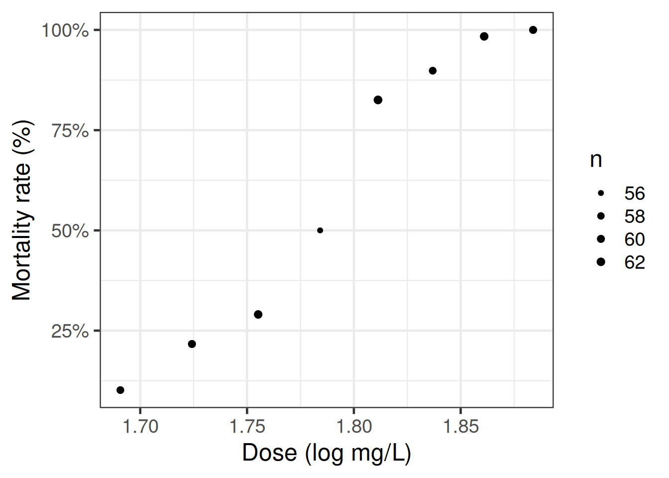
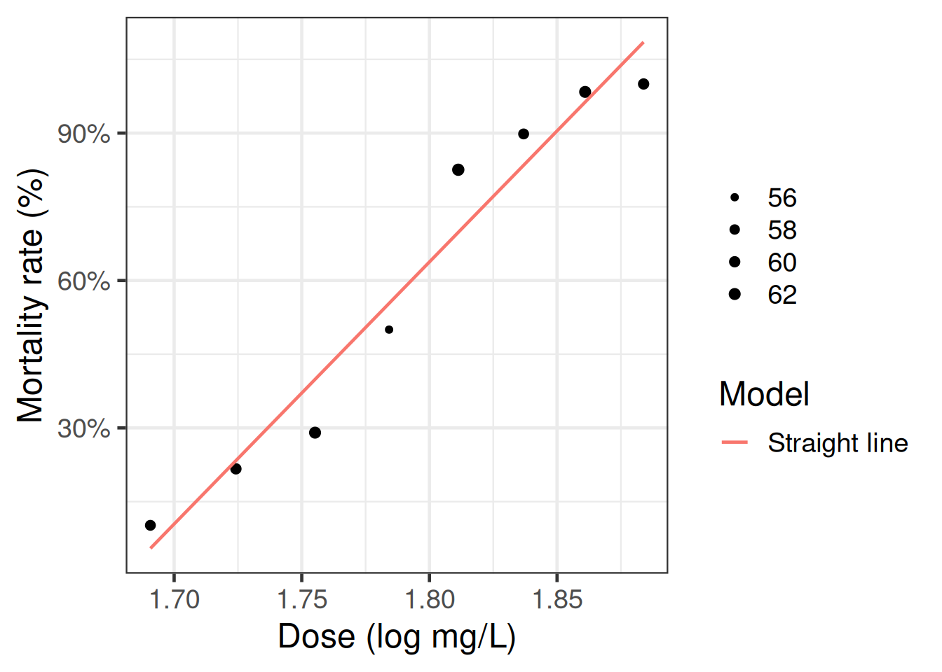
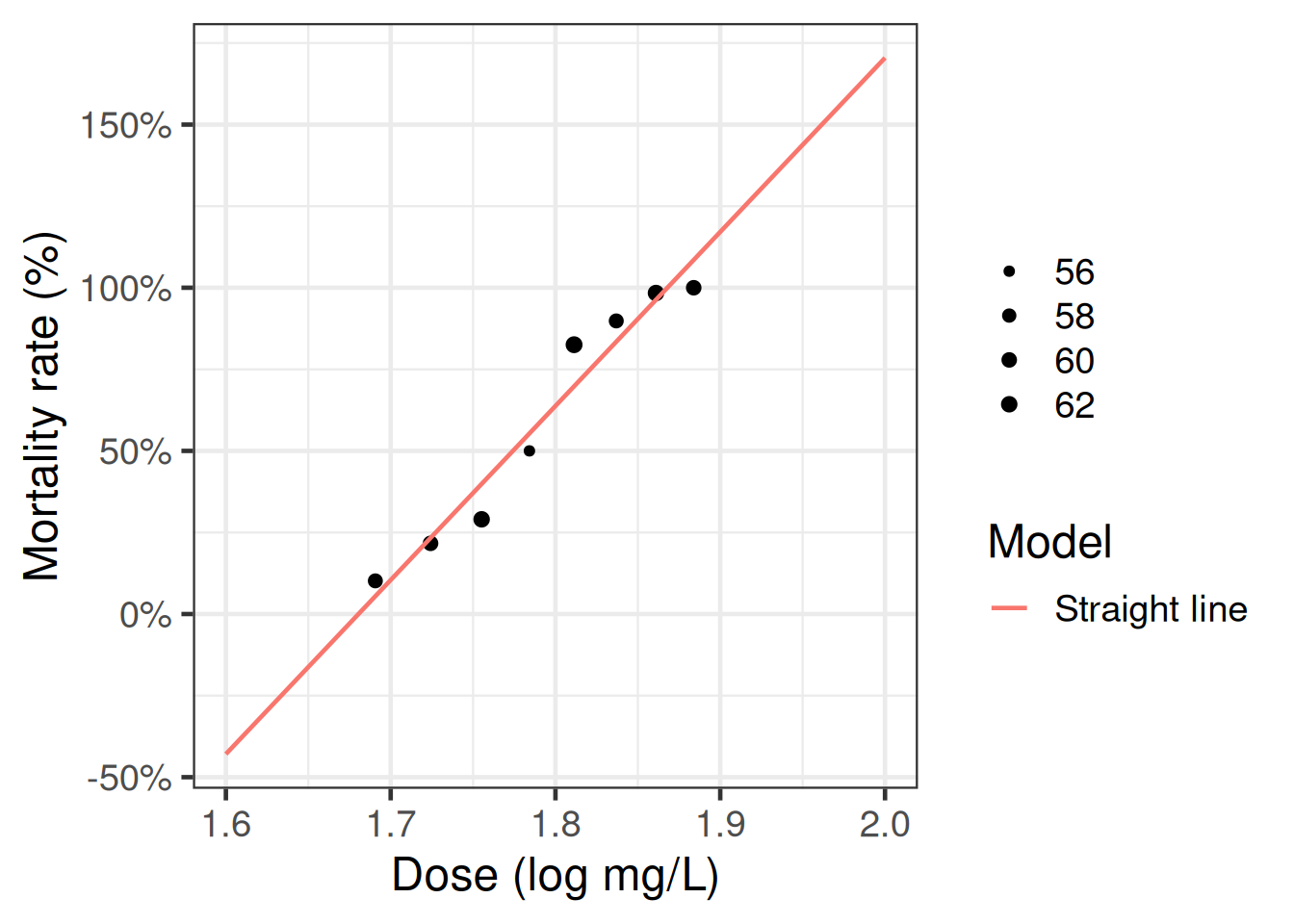
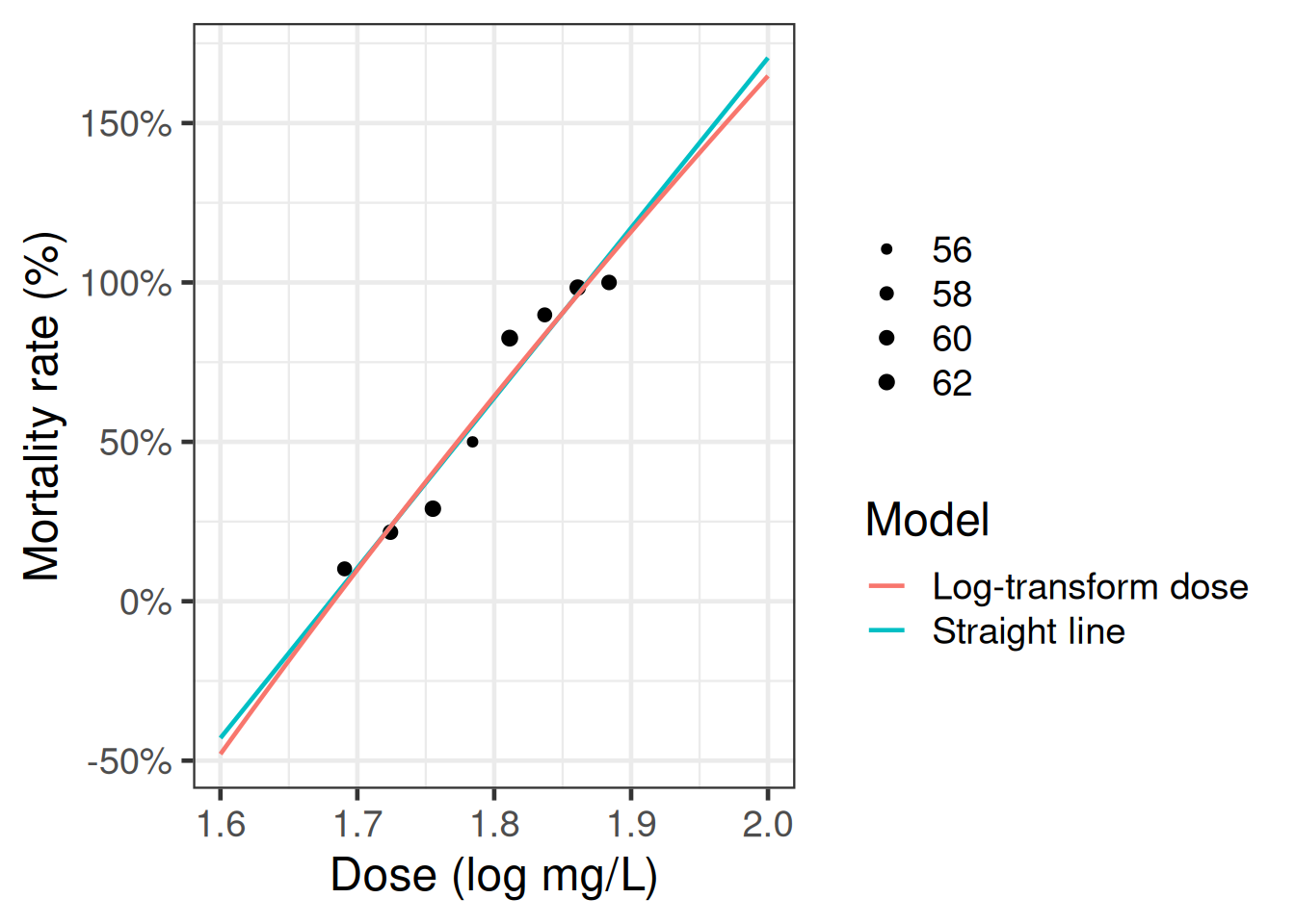
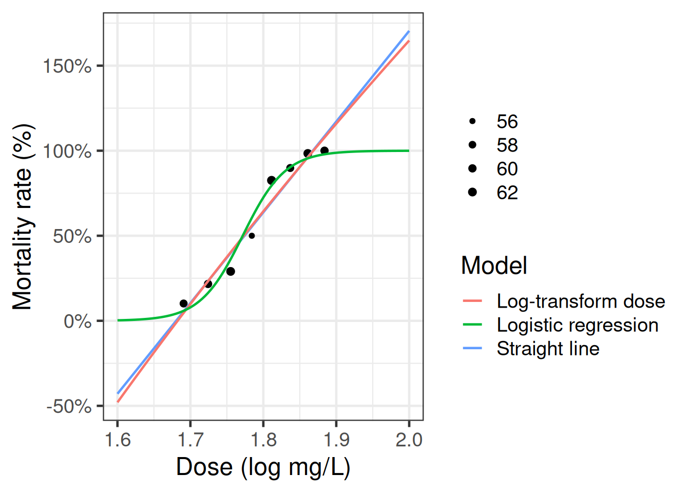
Example 9 In our model for the beetles data, we only have an intercept plus one covariate, gas concentration (\(c\)): \[\tilde{x}= (1, c)\]

If \(c_i\) is the gas concentration for the beetle in observation \(i\), and \(\tilde{c} = (c_1, c_2, ...c_n)\), then the score equation \(\tilde{\ell'} = 0\) means that for the MLE \(\hat{\tilde{\beta}}\):

1. the sum of the errors (aka deviations) equals 0:

\[\sum_{i=1}^n\varepsilon_i = 0\]

2. the weighted sum of the error times the gas concentrations equals 0:

\[\sum_{i=1}^nc_i \varepsilon_i = 0 \]

Exercise 36 Implement and graph the score function for the beetles data

Solution 30.

odds_inv <- function(omega) (1 + omega^-1)^-1

score_fn_beetles_beta0_0 <- function(beta_0, beta_1) {
  beetles |>
    mutate(
      eta = beta_0 + beta_1 * dose_c,
      omega = exp(eta),
      pi = odds_inv(omega),
      mu = pi * n,
      epsilon = died - mu,
      score = epsilon
    ) |>
    pull(score) |>
    sum()
}
score_fn_beetles_beta_0 <- Vectorize(score_fn_beetles_beta0_0)

score_fn_beetles_beta1_0 <- function(beta_0, beta_1) {
  beetles |>
    mutate(
      eta = beta_0 + beta_1 * dose_c,
      omega = exp(eta),
      pi = odds_inv(omega),
      mu = pi * n,
      epsilon = died - mu,
      score = dose_c * epsilon
    ) |>
    pull(score) |>
    sum()
}
score_fn_beetles_beta_1 <- Vectorize(score_fn_beetles_beta1_0)

if (run_graphs) {
  scores_beetles_beta_0 <- outer(beta_0s, beta_1s, score_fn_beetles_beta_0)
  scores_beetles_beta_1 <- outer(beta_0s, beta_1s, score_fn_beetles_beta_1)

  plotly::plot_ly(
    x = ~beta_0s,
    y = ~beta_1s
  ) |>
    plotly::add_markers(
      type = "scatter",
      x = coef(beetles_glm_grouped_centered)["(Intercept)"],
      y = coef(beetles_glm_grouped_centered)["dose_c"],
      z = 0,
      marker = list(color = "black"),
      name = "MLE"
    ) |>
    plotly::add_surface(
      z = ~ t(scores_beetles_beta_1),
      name = "score_beta_1",
      colorscale = list(c(0, 1), c("red", "green")),
      showscale = FALSE,
      contours = list(
        z = list(
          show = TRUE,
          start = -1,
          end = 1,
          size = .1
        )
      ),
      opacity = 0.75
    ) |>
    plotly::add_surface(
      z = ~ t(scores_beetles_beta_0),
      colorscale = list(c(0, 1), c("yellow", "blue")),
      showscale = FALSE,
      contours = list(
        z = list(
          show = TRUE,
          start = -14,
          end = 14,
          size = 2
        )
      ),
      opacity = 0.75,
      name = "score_beta_0"
    ) |>
    plotly::layout(legend = list(orientation = "h"))
}

Figure 16: score functions of beetles data (centered model), by parameter (\(\beta_0\) and \(\beta_1\)), with MLE marked in black.

Hessian function

\[ {\ell''(\tilde{\beta})} = \sum_{i=1}^n{\color{olive}\ell''_i(\tilde{\beta})} \tag{26}\]

\[ \begin{aligned} {\color{olive}\ell''_i(\tilde{\beta})} &= \frac{\partial}{\partial \tilde{\beta}^{\top}}\tilde{\ell_i'} \\ &= \frac{\partial}{\partial \tilde{\beta}^{\top}}\tilde{x}_i\varepsilon_i \\ &= \tilde{x}_i \frac{\partial}{\partial \tilde{\beta}^{\top}}\varepsilon_i \\ &= \tilde{x}_i {\color{violet}\varepsilon_i'} \end{aligned} \tag{27}\]

Theorem 26 Using Lemma 12 and Theorem 21:

\[ \begin{aligned} \frac{\partial \pi}{\partial \tilde{\beta}} &= {\color{red}\frac{\partial \eta}{\partial \tilde{\beta}}} {\color{blue}\frac{\partial \pi}{\partial \eta}} \\ &= {\color{red}\tilde{x}} {\color{blue}\pi(1-\pi)} \end{aligned} \]

Using Theorem 26:

\[ \begin{aligned} {\color{violet}\varepsilon'_i} &= \frac{\partial \varepsilon_i}{\partial \tilde{\beta}^{\top}} \\ &= \frac{\partial}{\partial \tilde{\beta}^{\top}}\varepsilon_i \\ &=\frac{\partial}{\partial \tilde{\beta}^{\top}}(y_i - \mu_i) \\ &= \frac{\partial}{\partial \tilde{\beta}^{\top}}y_i - \frac{\partial}{\partial \tilde{\beta}^{\top}}\mu_i \\ &= 0 - \frac{\partial}{\partial \tilde{\beta}^{\top}}\mu_i \\ &= -\frac{\partial \mu_i}{\partial \tilde{\beta}^{\top}} \\ &= -{\color{purple}\frac{\partial \pi_i}{\partial \tilde{\beta}^{\top}}} \\ &= - \pi_i (1-\pi_i) \tilde{x}_i^{\top} \\ &= - \text{Var}{\left(Y_i|X_i=x_i\right)} \tilde{x}_i^{\top} \end{aligned} \]

Returning to Equation 27:

\[ \begin{aligned} {\color{olive}\ell''_i(\tilde{\beta})} &= \tilde{x}_i {\color{violet}\varepsilon_i'} \\ &= {\color{olive}-\tilde{x}_i \text{Var}{\left(Y_i|X_i=x_i\right)} \tilde{x}_i^{\top}} \end{aligned} \tag{28}\]

Returning to Equation 26:

\[ \begin{aligned} {\ell''(\tilde{\beta})} &= \sum_{i=1}^n{\color{olive}\ell''_i(\tilde{\beta})} \\ &= {-\sum_{i=1}^n\tilde{x}_i \text{Var}{\left(Y_i|X_i=x_i\right)} \tilde{x}_i'} \\ &= {- \mathbf{X}^{\top}\mathbf{D}\mathbf{X}} \end{aligned} \tag{29}\]

where \(\mathbf{D} \stackrel{\text{def}}{=}\text{diag}(\text{Var}{\left(Y_i|X_i=x_i\right)})\) is the diagonal matrix whose \(i^{th}\) diagonal element is \(\text{Var}{\left(Y_i|X_i=x_i\right)}\).

Compare with the linear regression Hessian:

\[ \begin{aligned} \ell''(\tilde{\beta}) &= -\frac{1}{\sigma^2}\sum_{i=1}^n\tilde{x}_i \tilde{x}_i' \\ &= -\mathbf{X}^{\top} \mathbf{D}^{-1} \mathbf{X} \end{aligned} \tag{30}\]

Exercise 37 Determine the elements of the Hessian matrix for logistic regression.

Solution 31. The components of the Hessian are:

\[ \begin{aligned} \ell''(\beta) &= \frac{\partial^2}{\partial \beta^{\top} \partial \beta}{\ell} \\ &= \frac{\partial}{\partial \beta^{\top}}\ell' \\ &= \begin{bmatrix} \frac{\partial \ell'}{\partial \beta_0} & \frac{\partial \ell'}{\partial \beta_1} & \cdots & \frac{\partial \ell'}{\partial \beta_p} \end{bmatrix} \\ &= \begin{bmatrix} \frac{\partial^2 \ell}{\partial \beta_0^2} & \frac{\partial^2 \ell}{\partial \beta_0 \partial \beta_1} & \cdots & \frac{\partial^2 \ell}{\partial \beta_0 \partial \beta_p} \\ \frac{\partial^2 \ell}{\partial \beta_1 \partial \beta_0} & \frac{\partial^2 \ell}{\partial \beta_1^2} & \cdots & \frac{\partial^2 \ell}{\partial \beta_0 \partial \beta_p} \\ \vdots & \ddots & \ddots & \vdots \\ \frac{\partial^2 \ell}{\partial \beta_p \partial \beta_0} & \frac{\partial^2 \ell}{\partial \beta_p \partial \beta_1} & \cdots & \frac{\partial^2 \ell}{\partial \beta_p^2} \end{bmatrix} \end{aligned} \]

Exercise 38 Determine the Hessian for the beetles model.

Solution 32. In the beetles model, the Hessian is:

\[ \begin{aligned} \ell''(\beta) &= \begin{bmatrix} \frac{\partial \ell'}{\partial \beta_0} & \frac{\partial \ell'}{\partial \beta_1} \end{bmatrix} \\ &= \begin{bmatrix} \frac{\partial^2 \ell}{\partial \beta_0^2} & \frac{\partial^2 \ell}{\partial \beta_0 \partial \beta_1} \\ \frac{\partial^2 \ell}{\partial \beta_1 \partial \beta_0} & \frac{\partial^2 \ell}{\partial \beta_1^2} \end{bmatrix} \\ &= \begin{bmatrix} -\sum_{i=1}^n\pi_i(1-\pi_i) & -\sum_{i=1}^nc_i \pi_i(1-\pi_i) \\ -\sum_{i=1}^nc_i \pi_i(1-\pi_i) & -\sum_{i=1}^nc_i^2 \pi_i(1-\pi_i) \end{bmatrix} \end{aligned} \]

Setting \(\ell'(\tilde{\beta}; \tilde{y}) = 0\) gives us:

\[\sum_{i=1}^n{\left\{\tilde{x}_i(y_i - \text{expit}{\left\{\tilde{x}_i'\beta\right\}}) \right\}} = 0 \tag{31}\]

In general, the estimating equation \(\ell'(\tilde{\beta}; \tilde{y}) = 0\) cannot be solved analytically.

Instead, we can use the Newton-Raphson method:

\[ {\widehat{\theta}}^* \leftarrow {\widehat{\theta}}^* - {\left(\ell''{\left(\tilde{y};{\widehat{\theta}}^*\right)}\right)}^{-1} \ell'{\left(\tilde{y};{\widehat{\theta}}^*\right)} \]

We make an iterative series of guesses, and each guess helps us make the next guess better (i.e., higher log-likelihood). You can see some information about this process like so:

beetles_glm_ungrouped <-
  beetles_long |>
  glm(
    control = glm.control(trace = TRUE),
    formula = outcome ~ dose,
    family = "binomial"
  )
#> Deviance = 383.249 Iterations - 1
#> Deviance = 372.921 Iterations - 2
#> Deviance = 372.472 Iterations - 3
#> Deviance = 372.471 Iterations - 4
#> Deviance = 372.471 Iterations - 5

After each iteration of the fitting procedure, the deviance (\(2(\ell_{\text{full}} - \ell(\hat\beta))\) ) is printed. You can see that the algorithm took 5 iterations to converge to a solution where the likelihood wasn’t changing much anymore.

Table 12 and Table 13 show the fitted model and the covariance matrix of the estimates, respectively.

Table 12: Fitted model for beetles data

beetles_glm_ungrouped |> summary()
#> 
#> Call:
#> glm(formula = outcome ~ dose, family = "binomial", data = beetles_long, 
#>     control = glm.control(trace = TRUE))
#> 
#> Coefficients:
#>             Estimate Std. Error z value Pr(>|z|)    
#> (Intercept)   -60.72       5.18   -11.7   <2e-16 ***
#> dose           34.27       2.91    11.8   <2e-16 ***
#> ---
#> Signif. codes:  0 '***' 0.001 '**' 0.01 '*' 0.05 '.' 0.1 ' ' 1
#> 
#> (Dispersion parameter for binomial family taken to be 1)
#> 
#>     Null deviance: 645.44  on 480  degrees of freedom
#> Residual deviance: 372.47  on 479  degrees of freedom
#> AIC: 376.5
#> 
#> Number of Fisher Scoring iterations: 5

Table 13: Parameter estimate covariance matrix for beetles data

beetles_glm_ungrouped |> vcov()
#>             (Intercept)      dose
#> (Intercept)     26.8393 -15.08189
#> dose           -15.0819   8.48041

6 Inference for logistic regression models

6.1 Inference for individual predictor coefficients

Wald tests and confidence intervals

By the central limit theorem for MLEs, the maximum likelihood estimates \(\hat\beta_k\) are approximately Gaussian for large sample sizes; see also the table of Gaussian vs. MLE-based tests.

Wald test statistic

To test \(H_0: \beta_k = \beta_{k,0}\) (typically \(\beta_{k,0} = 0\)):

\[z_k = \frac{\hat\beta_k - \beta_{k,0}}{\widehat{SE}(\hat\beta_k)}\]

Under \(H_0\), \(z_k \overset{\cdot}{\sim} N(0,1)\) for large \(n\).

Confidence intervals for regression coefficients

A 95% confidence interval for \(\beta_k\) is:

\[\hat\beta_k \pm 1.96 \cdot \widehat{SE}(\hat\beta_k)\]

Confidence intervals for exponentiated coefficients

By the invariance property of MLEs, the MLE of \(e^{\beta_k}\) is \(e^{\hat\beta_k}\).

A 95% confidence interval for \(e^{\beta_k}\) is obtained by exponentiating the endpoints of the CI for \(\beta_k\):

\[e^{\beta_k} \in \left(e^{\hat\beta_k - 1.96 \cdot \widehat{SE}(\hat\beta_k)},\; e^{\hat\beta_k + 1.96 \cdot \widehat{SE}(\hat\beta_k)}\right)\]

For covariate coefficients (\(k \neq 0\)), \(e^{\beta_k}\) is an odds ratio (the multiplicative change in odds per 1-unit increase in \(x_k\), holding all other covariates fixed). For the intercept (\(k = 0\)), \(e^{\beta_0}\) is the baseline odds (the odds when all covariates equal zero), not an odds ratio.

In R

In R, parameters() from the parameters package automatically computes Wald tests and confidence intervals for logistic regression model coefficients:

beetles_glm_ungrouped |>
  parameters() |>
  print_md()
#> Deviance = 372.714 Iterations - 1
#> Deviance = 372.714 Iterations - 2
#> Deviance = 373.417 Iterations - 1
#> Deviance = 373.417 Iterations - 2
#> Deviance = 374.544 Iterations - 1
#> Deviance = 374.544 Iterations - 2
#> Deviance = 376.063 Iterations - 1
#> Deviance = 376.063 Iterations - 2
#> Deviance = 377.943 Iterations - 1
#> Deviance = 377.943 Iterations - 2
#> Deviance = 380.156 Iterations - 1
#> Deviance = 380.156 Iterations - 2
#> Deviance = 372.727 Iterations - 1
#> Deviance = 372.727 Iterations - 2
#> Deviance = 373.526 Iterations - 1
#> Deviance = 373.526 Iterations - 2
#> Deviance = 374.912 Iterations - 1
#> Deviance = 374.912 Iterations - 2
#> Deviance = 376.937 Iterations - 1
#> Deviance = 376.937 Iterations - 2
#> Deviance = 376.937 Iterations - 3
#> Deviance = 379.654 Iterations - 1
#> Deviance = 379.654 Iterations - 2
#> Deviance = 379.654 Iterations - 3
#> Deviance = 372.727 Iterations - 1
#> Deviance = 372.727 Iterations - 2
#> Deviance = 373.526 Iterations - 1
#> Deviance = 373.526 Iterations - 2
#> Deviance = 374.913 Iterations - 1
#> Deviance = 374.913 Iterations - 2
#> Deviance = 376.94 Iterations - 1
#> Deviance = 376.94 Iterations - 2
#> Deviance = 379.66 Iterations - 1
#> Deviance = 379.66 Iterations - 2
#> Deviance = 379.66 Iterations - 3
#> Deviance = 372.714 Iterations - 1
#> Deviance = 372.714 Iterations - 2
#> Deviance = 373.417 Iterations - 1
#> Deviance = 373.417 Iterations - 2
#> Deviance = 374.543 Iterations - 1
#> Deviance = 374.543 Iterations - 2
#> Deviance = 376.061 Iterations - 1
#> Deviance = 376.061 Iterations - 2
#> Deviance = 377.939 Iterations - 1
#> Deviance = 377.939 Iterations - 2
#> Deviance = 380.151 Iterations - 1
#> Deviance = 380.151 Iterations - 2

Table 14: Wald tests and 95% CIs for beetles logistic regression

Parameter	Log-Odds	SE	95% CI	z	p
(Intercept)	-60.72	5.18	(-71.44, -51.08)	-11.72	< .001
dose	34.27	2.91	(28.85, 40.30)	11.77	< .001

Pass exponentiate = TRUE to parameters() to report exponentiated coefficients. The intercept is then interpreted as baseline odds, while the non-intercept coefficients are odds ratios:

beetles_glm_ungrouped |>
  parameters(exponentiate = TRUE) |>
  print_md()
#> Deviance = 372.714 Iterations - 1
#> Deviance = 372.714 Iterations - 2
#> Deviance = 373.417 Iterations - 1
#> Deviance = 373.417 Iterations - 2
#> Deviance = 374.544 Iterations - 1
#> Deviance = 374.544 Iterations - 2
#> Deviance = 376.063 Iterations - 1
#> Deviance = 376.063 Iterations - 2
#> Deviance = 377.943 Iterations - 1
#> Deviance = 377.943 Iterations - 2
#> Deviance = 380.156 Iterations - 1
#> Deviance = 380.156 Iterations - 2
#> Deviance = 372.727 Iterations - 1
#> Deviance = 372.727 Iterations - 2
#> Deviance = 373.526 Iterations - 1
#> Deviance = 373.526 Iterations - 2
#> Deviance = 374.912 Iterations - 1
#> Deviance = 374.912 Iterations - 2
#> Deviance = 376.937 Iterations - 1
#> Deviance = 376.937 Iterations - 2
#> Deviance = 376.937 Iterations - 3
#> Deviance = 379.654 Iterations - 1
#> Deviance = 379.654 Iterations - 2
#> Deviance = 379.654 Iterations - 3
#> Deviance = 372.727 Iterations - 1
#> Deviance = 372.727 Iterations - 2
#> Deviance = 373.526 Iterations - 1
#> Deviance = 373.526 Iterations - 2
#> Deviance = 374.913 Iterations - 1
#> Deviance = 374.913 Iterations - 2
#> Deviance = 376.94 Iterations - 1
#> Deviance = 376.94 Iterations - 2
#> Deviance = 379.66 Iterations - 1
#> Deviance = 379.66 Iterations - 2
#> Deviance = 379.66 Iterations - 3
#> Deviance = 372.714 Iterations - 1
#> Deviance = 372.714 Iterations - 2
#> Deviance = 373.417 Iterations - 1
#> Deviance = 373.417 Iterations - 2
#> Deviance = 374.543 Iterations - 1
#> Deviance = 374.543 Iterations - 2
#> Deviance = 376.061 Iterations - 1
#> Deviance = 376.061 Iterations - 2
#> Deviance = 377.939 Iterations - 1
#> Deviance = 377.939 Iterations - 2
#> Deviance = 380.151 Iterations - 1
#> Deviance = 380.151 Iterations - 2

Table 15: Exponentiated coefficients and 95% CIs for beetles

Parameter	Odds Ratio	SE	95% CI	z	p
(Intercept)	4.27e-27	2.21e-26	(9.39e-32, 6.56e-23)	-11.72	< .001
dose	7.65e+14	2.23e+15	(3.40e+12, 3.18e+17)	11.77	< .001

6.2 Inference for predicted probabilities

Exercise 39 Given a maximum likelihood estimate \(\hat \beta\) and a corresponding estimated covariance matrix \(\hat \Sigma\stackrel{\text{def}}{=}\widehat{\text{Cov}}(\hat \beta)\), calculate a 95% confidence interval for the predicted probability \(\pi(\tilde{x}) = \Pr(Y = 1 | \tilde{X}= \tilde{x})\).

Solution 33.

By the central limit theorem for MLEs, a 95% confidence interval for \(\pi(\tilde{x})\) can be constructed as:

\[\hat\pi(\tilde{x}) \pm 1.96 * \widehat{\text{SE}}{\left(\hat\pi(\tilde{x})\right)}\]

However, \(\widehat{\text{SE}}{\left(\hat\pi(\tilde{x})\right)}\) seems difficult to compute; doing so would require using the delta method.

Instead, using the invariance property of MLEs, we can first calculate a confidence interval for the log-odds,

\[\eta(\tilde{x}) = \tilde{x}'\tilde{\beta}\in (L, R)\]

and then apply \(\text{expit}\) to the endpoints of that log-odds-scale confidence interval:

\[\pi(\tilde{x}) \in (\text{expit}(L), \text{expit}(R)) \tag{32}\]

Exercise 40 Find a 95% confidence interval for the log-odds \(\eta(\tilde{x}) = \tilde{x}'\tilde{\beta}\).

Solution 34. By the central limit theorem for MLEs, a 95% confidence interval for \(\eta(\tilde{x})\) can be constructed as:

\[\hat\eta(\tilde{x}) \pm 1.96 * {\color{blue}\widehat{\text{SE}}{\left(\hat\eta(\tilde{x})\right)}}\]

where \(\hat\eta(\tilde{x}) = \tilde{x}'\hat \beta\).

Exercise 41  

How can we estimate the standard error of \(\hat\eta(\tilde{x})\)?

\[{\color{blue}\widehat{\text{SE}}{\left(\hat\eta(\tilde{x})\right)}} = {\color{blue}?}\]

Solution 35. \[ {\color{green}\text{SE}{\left(\hat\eta(\tilde{x})\right)}} = \sqrt{{\color{red}\text{Var}{\left(\hat\eta(\tilde{x})\right)}}} \tag{33}\]

By the definition \(\hat\eta(\tilde{x}) = \tilde{x}'\hat \beta\) and the variance of a linear combination:

\[ \begin{aligned} {\color{red}\text{Var}{\left(\hat\eta(\tilde{x})\right)}} &= \text{Var}{\left(\tilde{x}'\hat \beta\right)} \\ &= \tilde{x}'\text{Cov}{\left(\hat \beta\right)}\tilde{x} \\ &= {\color{red}{\tilde{x}}^{\top}\Sigma\tilde{x}} \end{aligned} \tag{34}\]

where \(\Sigma \stackrel{\text{def}}{=}\text{Cov}(\hat \beta)\).

---

Expanding Equation 34 out of matrix-vector notation, we have:

\[ \begin{aligned} {\color{red}{\tilde{x}}^{\top}\Sigma\tilde{x}} &= \sum_{i=1}^p\sum_{j=1}^px_i \Sigma_{ij} x_j \\ &= {\color{red}\sum_{i=1}^p\sum_{j=1}^px_i \text{Cov}(\hat \beta_i,\hat \beta_j) x_j} \end{aligned} \]

---

Combining Equation 34 and MLE invariance:

Theorem 27 (Estimated variance and standard error of log-odds) \[ {\color{orange}\widehat{\text{Var}}{\left(\hat\eta(\tilde{x})\right)}} = {\color{orange}{\tilde{x}}^{\top}\hat{\Sigma}\tilde{x}} \tag{35}\]

\[ {\color{blue}\widehat{\text{SE}}{\left(\hat\eta(\tilde{x})\right)}} = {\color{blue}\sqrt{{\tilde{x}}^{\top}\hat{\Sigma}\tilde{x}}} \tag{36}\]

Note: on the RHS, we have plugged in \(\hat{\Sigma}\), our estimate of \(\Sigma\).

In R

In R, predict() with type = "link" and se.fit = TRUE computes the estimated log-odds \(\hat\eta(\tilde{x}) = \tilde{x}'\hat \beta\) and its estimated standard error for each covariate pattern:

library(dplyr)
new_doses <- tibble(dose = c(1.7, 1.8, 1.9))

pred_logodds <-
  beetles_glm_ungrouped |>
  predict(
    newdata = new_doses,
    type = "link",
    se.fit = TRUE
  )

new_doses |>
  mutate(
    logodds_hat = pred_logodds$fit,
    se = pred_logodds$se.fit,
    ci_lower_logodds = logodds_hat - 1.96 * se,
    ci_upper_logodds = logodds_hat + 1.96 * se,
    pi_hat = plogis(logodds_hat),
    ci_lower_prob = plogis(ci_lower_logodds),
    ci_upper_prob = plogis(ci_upper_logodds)
  ) |>
  knitr::kable(digits = 3)

Table 16: Predicted log-odds and 95% CI for beetles logistic regression

dose	logodds_hat	se	ci_lower_logodds	ci_upper_logodds	pi_hat	ci_lower_prob	ci_upper_prob
1.7	-2.458	0.263	-2.974	-1.942	0.079	0.049	0.125
1.8	0.969	0.145	0.685	1.253	0.725	0.665	0.778
1.9	4.396	0.377	3.656	5.136	0.988	0.975	0.994

6.3 Inference for odds ratios

Exercise 42 Given a maximum likelihood estimate \(\hat \beta\) and a corresponding estimated covariance matrix \(\hat \Sigma\stackrel{\text{def}}{=}\widehat{\text{Cov}}(\hat \beta)\), calculate a 95% confidence interval for the odds ratio comparing covariate patterns \(\tilde{x}\) and \({\tilde{x}^*}\), \(\theta(\tilde{x},{\tilde{x}^*})\).

Solution 36.

By the central limit theorem for MLEs, a 95% confidence interval for \(\theta(\tilde{x},{\tilde{x}^*})\) can be constructed as:

\[\hat\theta\pm 1.96 * \widehat{\text{SE}}{\left(\hat\theta\right)} \tag{37}\] However, \(\widehat{\text{SE}}{\left(\hat\theta\right)}\) seems difficult to compute; doing so would require using the delta method.

Instead, using the invariance property of MLEs, we can first calculate a confidence interval for the logarithm of the odds ratio,

\[\text{log}{\left\{\theta(\tilde{x},{\tilde{x}^*})\right\}} \in (L,R) \tag{38}\]

and then exponentiate the endpoints of that log-odds-scale confidence interval:

\[\theta(\tilde{x},{\tilde{x}^*}) \in (e^L, e^R) \tag{39}\]

Exercise 43 Find a 95% confidence interval for the natural logarithm of the odds ratio, \(\text{log}{\left\{\theta(\tilde{x},{\tilde{x}^*})\right\}}\)

Solution 37. From Corollary 12, we know:

\[\text{log}{\left\{\theta(\tilde{x},{\tilde{x}^*})\right\}} = \Delta \eta\]

By the central limit theorem for MLEs, a 95% confidence interval for \(\Delta \eta\) can be constructed as:

\[\widehat{\Delta \eta}\pm 1.96 * {\color{blue}\widehat{\text{SE}}{\left(\widehat{\Delta \eta}\right)}}\]

Exercise 44  

How can we estimate the standard error of \(\widehat{\Delta \eta}\)?

\[{\color{blue}\widehat{\text{SE}}{\left(\widehat{\Delta \eta}\right)}} = {\color{blue}?}\]

Solution 38. \[ {\color{green}\text{SE}{\left(\widehat{\Delta \eta}\right)}} = \sqrt{{\color{red}\text{Var}{\left(\widehat{\Delta \eta}\right)}}} \tag{40}\]

By Lemma 8 and the variance of a linear combination:

\[ \begin{aligned} {\color{red}\text{Var}{\left(\widehat{\Delta \eta}\right)}} &= \text{Var}{\left((\Delta\tilde{x}) \cdot \hat \beta\right)} \\ &= {\left(\Delta\tilde{x}\right)}^{\top}\text{Cov}{\left(\hat \beta\right)}(\Delta\tilde{x}) \\ &= {\color{red}{\left(\Delta\tilde{x}\right)}^{\top}\Sigma(\Delta\tilde{x})} \end{aligned} \tag{41}\]

where \(\Sigma \stackrel{\text{def}}{=}\text{Cov}(\hat \beta)\).

---

Expanding Equation 41 out of matrix-vector notation, we have:

\[ \begin{aligned} {\color{red}{\left(\Delta\tilde{x}\right)}^{\top}\Sigma(\Delta\tilde{x})} &= \sum_{i=1}^p\sum_{j=1}^p(\Delta\tilde{x})_i \Sigma_{ij} (\Delta\tilde{x})_j \\ &= \sum_{i=1}^p\sum_{j=1}^p(\Delta x_i) \Sigma_{ij} (\Delta x_j) \\ &= {\color{red}\sum_{i=1}^p\sum_{j=1}^p(x_i - x^*_i) \text{Cov}(\hat \beta_i,\hat \beta_j) (x_j - x^*_j)} \end{aligned} \]

---

Combining Equation 41 and MLE invariance:

Theorem 28 (Estimated variance and standard error of difference in log-odds) \[ {\color{orange}\widehat{\text{Var}}{\left(\Delta{\hat\eta}\right)}} = {\color{orange}{\Delta\tilde{x}}^{\top}\hat{\Sigma}(\Delta\tilde{x})} \tag{42}\]

\[ {\color{blue}\widehat{\text{SE}}{\left(\Delta{\hat\eta}\right)}} = {\color{blue}\sqrt{{\Delta\tilde{x}}^{\top}\hat{\Sigma}(\Delta\tilde{x})}} \tag{43}\]

Note: on the RHS, we have plugged in \(\hat{\Sigma}\), our estimate of \(\Sigma\).

Compare this result with confidence intervals.

7 Multiple logistic regression

Coronary heart disease (WCGS) study data

Let’s use the data from the Western Collaborative Group Study (WCGS) (Rosenman et al. (1975)) to explore multiple logistic regression:

From Vittinghoff et al. (2012):

“The Western Collaborative Group Study (WCGS) was a large epidemiological study designed to investigate the association between the”type A” behavior pattern and coronary heart disease (CHD)“.

Exercise 45 What is “type A” behavior?

Solution 39. From Wikipedia, “Type A and Type B personality theory”:

“The hypothesis describes Type A individuals as outgoing, ambitious, rigidly organized, highly status-conscious, impatient, anxious, proactive, and concerned with time management….

The hypothesis describes Type B individuals as a contrast to those of Type A. Type B personalities, by definition, are noted to live at lower stress levels. They typically work steadily and may enjoy achievement, although they have a greater tendency to disregard physical or mental stress when they do not achieve.”

Study design

from ?faraway::wcgs:

3154 healthy young men aged 39-59 from the San Francisco area were assessed for their personality type. All were free from coronary heart disease at the start of the research. Eight and a half years later change in CHD status was recorded.

Details (from faraway::wcgs)

The WCGS began in 1960 with 3,524 male volunteers who were employed by 11 California companies. Subjects were 39 to 59 years old and free of heart disease as determined by electrocardiogram. After the initial screening, the study population dropped to 3,154 and the number of companies to 10 because of various exclusions. The cohort comprised both blue- and white-collar employees.

Baseline data collection

socio-demographic characteristics:

• age
• education
• marital status
• income
• occupation
• physical and physiological including:
• height
• weight
• blood pressure
• electrocardiogram
• corneal arcus

biochemical measurements:

• cholesterol and lipoprotein fractions;
• medical and family history and use of medications;

behavioral data:

• Type A interview,
• smoking,
• exercise
• alcohol use.

Later surveys added data on:

• anthropometry
• triglycerides
• Jenkins Activity Survey
• caffeine use

Average follow-up continued for 8.5 years with repeat examinations.

Load the data

Here, I load the data:

### load the data directly from a UCSF website:
library(haven)
url <- paste0(
  # I'm breaking up the url into two chunks for readability
  "https://regression.ucsf.edu/sites/g/files/",
  "tkssra6706/f/wysiwyg/home/data/wcgs.dta"
)
wcgs <- haven::read_dta(url)

wcgs

Table 17: wcgs data

Data cleaning

Now let’s do some data cleaning

library(arsenal) # provides `set_labels()`
library(forcats) # provides `as_factor()`
library(haven)
library(plotly)
wcgs <- wcgs |>
  mutate(
    age = age |>
      arsenal::set_labels("Age (years)"),
    arcus = arcus |>
      as.logical() |>
      arsenal::set_labels("Arcus Senilis"),
    time169 = time169 |>
      as.numeric() |>
      arsenal::set_labels("Observation (follow up) time (days)"),
    dibpat = dibpat |>
      as_factor() |>
      relevel(ref = "Type B") |>
      arsenal::set_labels("Behavioral Pattern"),
    typchd69 = typchd69 |>
      labelled(
        label = "Type of CHD Event",
        labels =
          c(
            "None" = 0,
            "infdeath" = 1,
            "silent" = 2,
            "angina" = 3
          )
      ),

    # turn stata-style labelled variables in to R-style factors:
    across(
      where(is.labelled),
      haven::as_factor
    )
  )

What’s in the data

Table 18 summarizes the data.

library(gtsummary)
wcgs |>
  dplyr::select(
    -dplyr::all_of(c("id", "uni", "t1"))
  ) |>
  gtsummary::tbl_summary(
    by = "chd69",
    missing_text = "Missing"
  ) |>
  gtsummary::add_p() |>
  gtsummary::add_overall() |>
  gtsummary::bold_labels() |> 
  gtsummary::separate_p_footnotes()

Table 18: Baseline characteristics by CHD status at end of follow-up

Characteristic	Overall N = 3,1541	No N = 2,8971	Yes N = 2571	p-value
Age (years)	45.0 (42.0, 50.0)	45.0 (41.0, 50.0)	49.0 (44.0, 53.0)	<0.0012
Arcus Senilis	941 (30%)	839 (29%)	102 (40%)	<0.0013
Missing	2	0	2
Behavioral Pattern				<0.0013
A1	264 (8.4%)	234 (8.1%)	30 (12%)
A2	1,325 (42%)	1,177 (41%)	148 (58%)
B3	1,216 (39%)	1,155 (40%)	61 (24%)
B4	349 (11%)	331 (11%)	18 (7.0%)
Body Mass Index (kg/m2)	24.39 (22.96, 25.84)	24.39 (22.89, 25.84)	24.82 (23.63, 26.50)	<0.0012
Total Cholesterol	223 (197, 253)	221 (195, 250)	245 (222, 276)	<0.0012
Missing	12	12	0
Diastolic Blood Pressure	80 (76, 86)	80 (76, 86)	84 (80, 90)	<0.0012
Behavioral Pattern				<0.0013
Type B	1,565 (50%)	1,486 (51%)	79 (31%)
Type A	1,589 (50%)	1,411 (49%)	178 (69%)
Height (inches)	70.00 (68.00, 72.00)	70.00 (68.00, 72.00)	70.00 (68.00, 71.00)	0.42
Ln of Systolic Blood Pressure	4.84 (4.79, 4.91)	4.84 (4.77, 4.91)	4.87 (4.82, 4.97)	<0.0012
Ln of Weight	5.14 (5.04, 5.20)	5.13 (5.04, 5.20)	5.16 (5.09, 5.22)	<0.0012
Cigarettes per day	0 (0, 20)	0 (0, 20)	20 (0, 30)	<0.0012
Systolic Blood Pressure	126 (120, 136)	126 (118, 136)	130 (124, 144)	<0.0012
Current smoking	1,502 (48%)	1,343 (46%)	159 (62%)	<0.0013
Observation (follow up) time (days)	2,942 (2,842, 3,037)	2,952 (2,864, 3,048)	1,666 (934, 2,400)	<0.0012
Type of CHD Event				<0.0014
None	0 (0%)	0 (0%)	0 (0%)
infdeath	2,897 (92%)	2,897 (100%)	0 (0%)
silent	135 (4.3%)	0 (0%)	135 (53%)
angina	71 (2.3%)	0 (0%)	71 (28%)
4	51 (1.6%)	0 (0%)	51 (20%)
Weight (lbs)	170 (155, 182)	169 (155, 182)	175 (162, 185)	<0.0012
Weight Category				<0.0013
< 140	232 (7.4%)	217 (7.5%)	15 (5.8%)
140-170	1,538 (49%)	1,440 (50%)	98 (38%)
170-200	1,171 (37%)	1,049 (36%)	122 (47%)
> 200	213 (6.8%)	191 (6.6%)	22 (8.6%)
RECODE of age (Age)				<0.0013
35-40	543 (17%)	512 (18%)	31 (12%)
41-45	1,091 (35%)	1,036 (36%)	55 (21%)
46-50	750 (24%)	680 (23%)	70 (27%)
51-55	528 (17%)	463 (16%)	65 (25%)
56-60	242 (7.7%)	206 (7.1%)	36 (14%)
1 Median (Q1, Q3); n (%)
2 Wilcoxon rank sum test
3 Pearson’s Chi-squared test
4 Fisher’s exact test

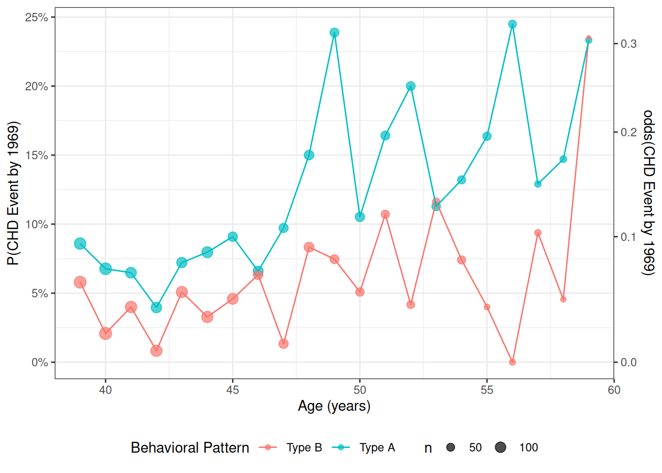
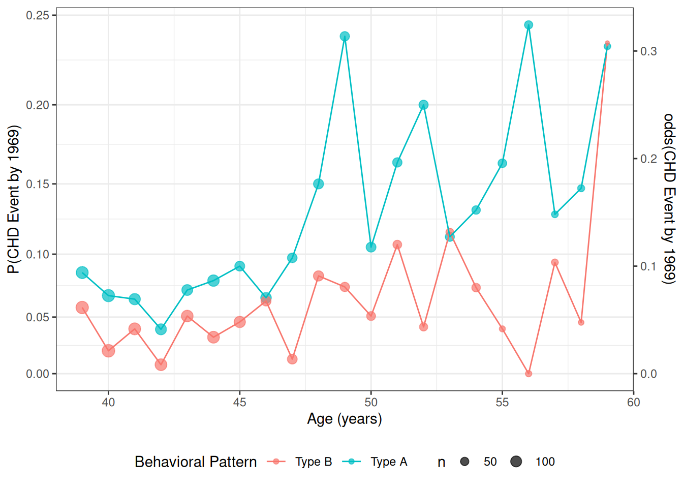
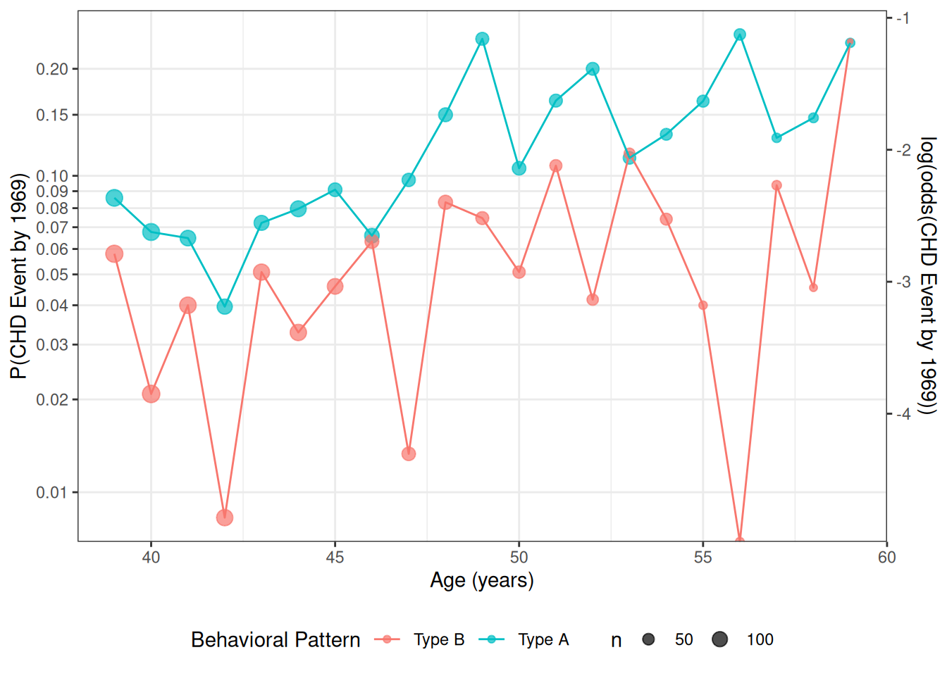
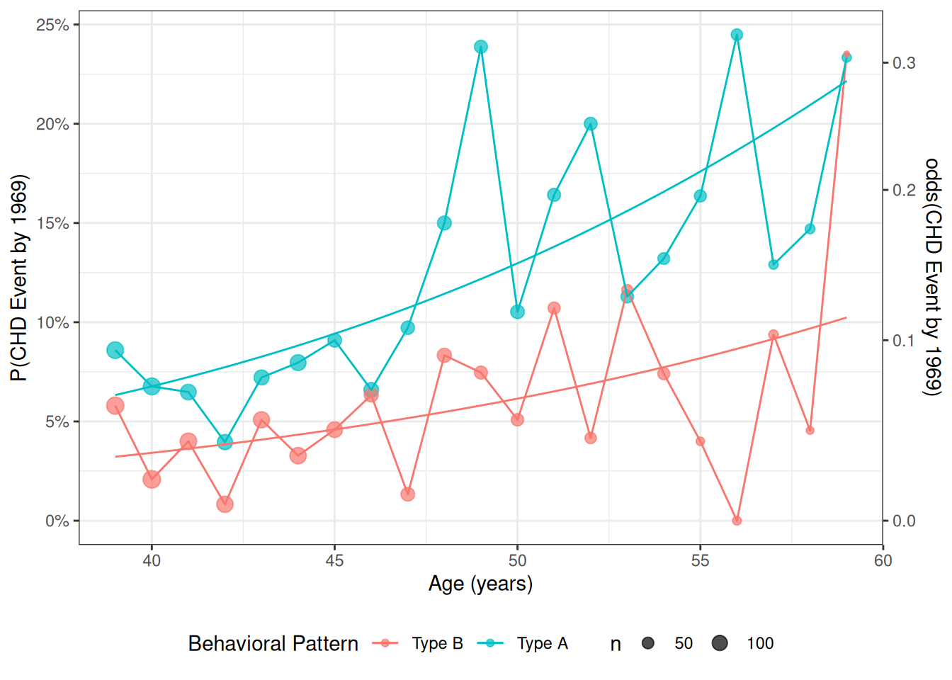
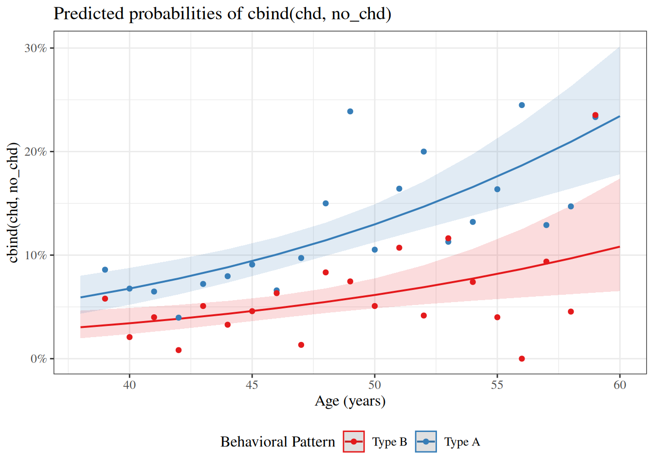
Data by age and personality type

For now, we will look at the interaction between age and personality type (dibpat). To make it easier to visualize the data, we summarize the event rates for each combination of age:

library(dplyr)
odds <- function(pi) pi / (1 - pi)
chd_grouped_data <-
  wcgs |>
  summarize(
    .by = c(age, dibpat),
    n = sum(chd69 %in% c("Yes", "No")),
    x = sum(chd69 == "Yes")
  ) |>
  mutate(
    `n - x` = n - x,
    `p(chd)` = (x / n) |>
      labelled(label = "CHD Event by 1969"),
    `odds(chd)` = `p(chd)` / (1 - `p(chd)`),
    `logit(chd)` = log(`odds(chd)`)
  )

chd_grouped_data

Graphical exploration

library(ggplot2)
library(scales)
chd_plot_probs <-
  chd_grouped_data |>
  ggplot() +
  aes(
    x = age,
    y = `p(chd)`,
    col = dibpat
  ) +
  geom_point(aes(size = n), alpha = .7) +
  scale_size(range = c(1, 4)) +
  geom_line() +
  theme_bw() +
  ylab("P(CHD Event by 1969)") +
  scale_y_continuous(
    labels = scales::label_percent(),
    sec.axis = sec_axis(
      ~ odds(.),
      name = "odds(CHD Event by 1969)"
    )
  ) +
  theme(legend.position = "bottom")

print(chd_plot_probs)

Figure 17: CHD rates by age group, probability scale

Odds scale

odds_inv <- function(omega) omega / (1 + omega)
trans_odds <- trans_new(
  name = "odds",
  transform = odds,
  inverse = odds_inv
)

chd_plot_odds <- chd_plot_probs +
  scale_y_continuous(
    trans = trans_odds, # this line changes the vertical spacing
    name = chd_plot_probs$labels$y,
    sec.axis = sec_axis(
      ~ odds(.),
      name = "odds(CHD Event by 1969)"
    )
  )

print(chd_plot_odds)

Figure 18: CHD rates by age group, odds spacing

Log-odds (logit) scale

logit <- function(pi) log(odds(pi))
expit <- function(eta) odds_inv(exp(eta))
trans_logit <- trans_new(
  name = "logit",
  transform = logit,
  inverse = expit
)

chd_plot_logit <-
  chd_plot_probs +
  scale_y_continuous(
    trans = trans_logit, # this line changes the vertical spacing
    name = chd_plot_probs$labels$y,
    breaks = c(seq(.01, .1, by = .01), .15, .2),
    minor_breaks = NULL,
    sec.axis = sec_axis(
      ~ logit(.),
      name = "log(odds(CHD Event by 1969))"
    )
  )

print(chd_plot_logit)

Figure 19: CHD data (logit-scale)

Logistic regression models for CHD data

For the wgcs dataset, let’s consider a logistic regression model for the outcome of Coronary Heart Disease (\(Y\); chd in computer output):

• \(Y = 1\) if an individual developed CHD by the end of the study;
• \(Y = 0\) if they have not developed CHD by the end of the study.

Let’s include an intercept, two covariates, plus their interaction:

• \(A\): age at study enrollment (age, recorded in years)
• \(P\): personality type (dibpat):
  • \(P = 1\) represents “Type A personality”,
  • \(P = 0\) represents “Type B personality”.
• \(PA\): the interaction of personality type and age (dibpat:age)
• \(\tilde{X}= (1, A, P, PA)\)

chd_glm_contrasts <-
  wcgs |>
  glm(
    "data" = _,
    "formula" = chd69 == "Yes" ~ dibpat * age,
    "family" = binomial(link = "logit")
  )

library(equatiomatic)
equatiomatic::extract_eq(chd_glm_contrasts)

\[ \log\left[ \frac { P( \operatorname{chd69} = \operatorname{Yes} ) }{ 1 - P( \operatorname{chd69} = \operatorname{Yes} ) } \right] = \alpha + \beta_{1}(\operatorname{dibpat}_{\operatorname{Type\ A}}) + \beta_{2}(\operatorname{age}) + \beta_{3}(\operatorname{dibpat}_{\operatorname{Type\ A}} \times \operatorname{age}) \]

Or in more formal notation:

\[ \begin{aligned} Y_i | \tilde{X}_i &\ \sim_{\perp\!\!\!\perp}\ \text{Ber}(\pi(\tilde{X}_i)) \\ \pi(\tilde{x}) &= \text{expit}(\eta(\tilde{x})) \\ \eta(\tilde{x}) &= \beta_0 + \beta_P p + \beta_A a + \beta_{PA} pa \end{aligned} \tag{44}\]

Models superimposed on data

We can graph our fitted models on each scale (probability, odds, log-odds).

probability scale

curve_type_A <- function(x) { # nolint: object_name_linter
  chd_glm_contrasts |> predict(
    type = "response",
    newdata = tibble(age = x, dibpat = "Type A")
  )
}

curve_type_B <- function(x) { # nolint: object_name_linter
  chd_glm_contrasts |> predict(
    type = "response",
    newdata = tibble(age = x, dibpat = "Type B")
  )
}

chd_plot_probs_2 <-
  chd_plot_probs +
  geom_function(
    fun = curve_type_A,
    aes(col = "Type A")
  ) +
  geom_function(
    fun = curve_type_B,
    aes(col = "Type B")
  )
print(chd_plot_probs_2)

chd_plot_odds_2 <-
  chd_plot_odds +
  geom_function(
    fun = curve_type_A,
    aes(col = "Type A")
  ) +
  geom_function(
    fun = curve_type_B,
    aes(col = "Type B")
  )
print(chd_plot_odds_2)

odds scale

log-odds (logit) scale

chd_plot_logit_2 <-
  chd_plot_logit +
  geom_function(
    fun = curve_type_A,
    aes(col = "Type A")
  ) +
  geom_function(
    fun = curve_type_B,
    aes(col = "Type B")
  )

print(chd_plot_logit_2)

Figure 20

Interpreting the model parameters

Exercise 46 For Equation 44, derive interpretations of \(\beta_0\), \(\beta_P\), \(\beta_A\), and \(\beta_{PA}\) on the odds and log-odds scales, State the interpretations concisely in math and in words.

Solution 40.  

# include: false
age_offset = 0L

\[ \begin{aligned} \eta(P=0,A=0) &= \beta_0 + \beta_P 0 + \beta_A 0 \\ &= \beta_0 + 0 + 0 \\ &= \beta_0 \end{aligned} \]

Therefore:

\[\beta_{0} = \eta(P=0,A=0) \tag{45}\]

\(\beta_{0}\) is the natural logarithm of the odds (“log-odds”) of experiencing CHD for a 0 year-old person with a type B personality; that is,

---

\(\text{e}^{\beta_{0}}\) is the odds of experiencing CHD for a 0 year-old with a type B personality,

\[ \begin{aligned} \text{exp}{\left\{\beta_{0}\right\}} &= \frac{\Pr(Y= 1| P = 0, A = 0)}{1-\Pr(Y= 1| P = 0, A = 0)} \\ &= \frac {\Pr(Y= 1| P = 0, A = 0)} {\Pr(Y= 0| P = 0, A = 0)} \end{aligned} \]

---

\[ \begin{aligned} \frac{\partial}{\partial a}\eta(P=0, A = a) &= \frac{\partial}{\partial a} (\beta_0 + \beta_P 0 + \beta_A a + \beta_{PA}(0\cdot a)) \\ &= \frac{\partial}{\partial a}\beta_0 + \frac{\partial}{\partial a}\beta_P 0 + \frac{\partial}{\partial a}\beta_A a + \frac{\partial}{\partial a}\beta_{PA}(0\cdot a)) \\ &= 0 + 0 + \beta_A + 0 \\ &= \beta_A \end{aligned} \]

Therefore:

\[\beta_A = \frac{\partial}{\partial a}\eta(P=0, A = a) \tag{46}\]

\(\beta_A\) is the slope of the log-odds of CHD with respect to age, for individuals with personality type B.

Alternatively:

\[ \begin{aligned} \beta_{A} &= \eta(P = 0, A = a + 1)- \eta(P = 0, A = a) \end{aligned} \]

That is, \(\beta_{A}\) is the difference in log-odds of experiencing CHD experiencing CHD per one-year difference in age between two individuals with type B personalities.

---

\[ \begin{aligned} \text{exp}{\left\{\beta_{A}\right\}} &= \text{exp}{\left\{\eta(P = 0, A = a + 1)- \eta(P = 0, A = a)\right\}} \\ &= \frac{\text{exp}{\left\{\eta(P = 0, A = a + 1)\right\}}}{\text{exp}{\left\{\eta(P = 0, A = a)\right\}}} \\ &= \frac{\omega(P = 0, A = a + 1)}{\omega(P = 0, A = a)} \\ &= \frac {\text{odds}(Y= 1|P=0, A = a + 1)} {\text{odds}(Y= 1|P=0, A = a)} \\ &= \theta(\Delta a = 1 | P = 0) \end{aligned} \]

• The odds ratio of experiencing CHD (aka “the odds ratio”) differs by a factor of \(\text{e}^{\beta_{A}}\) per one-year difference in age between individuals with type B personality.

---

\(\beta_{P}\) is the difference in log-odds of experiencing CHD for a 0 year-old person with type A personality compared to a 0 year-old person with type B personality; that is,

\[\beta_P = \eta(P = 1, A = 0) - \eta(P=0, A = 0) \tag{47}\]

---

• \(\text{e}^{\beta_{P}}\) is the ratio of the odds (aka “the odds ratio”) of experiencing CHD, for a 0-year old individual with type A personality vs a 0-year old individual with type B personality; that is,

\[ \text{exp}{\left\{\beta_{P}\right\}} = \frac {\text{odds}(Y= 1|P=1, A = 0)} {\text{odds}(Y= 1|P=0, A = 0)} \]

---

\[ \begin{aligned} \frac{\partial}{\partial a}\eta(P={\color{red}1}, A = a) &= {\color{red}\beta_A + \beta_{PA}} \\ \frac{\partial}{\partial a}\eta(P={\color{blue}0}, A = a) &= {\color{blue}\beta_A} \end{aligned} \]

Therefore:

\[ \begin{aligned} \frac{\partial}{\partial a}\eta(P={\color{red}1}, A = a) - \frac{\partial}{\partial a}\eta(P={\color{blue}0}, A = a) &= {\color{red}\beta_A + \beta_{PA}} - {\color{blue}\beta_A} \\ &= \beta_{PA} \end{aligned} \]

That is,

\[ \begin{aligned} \beta_{PA} &= \frac{\partial}{\partial a}\eta(P={\color{red}1}, A = a) - \frac{\partial}{\partial a}\eta(P={\color{blue}0}, A = a) \\ &= \frac{\partial}{\partial a}\eta(P={\color{red}1}, A = a) - \frac{\partial}{\partial a}\eta(P={\color{blue}0}, A = a) \end{aligned} \]

\(\beta_{PA}\) is the difference in the slopes of log-odds over age between participants with Type A personalities and participants with Type B personalities.

---

Accordingly, the odds ratio of experiencing CHD per one-year difference in age differs by a factor of \(\text{e}^{\beta_{PA}}\) for participants with type A personality compared to participants with type B personality; that is,

\[ \begin{aligned} \theta(\Delta a = 1 | P = 1) = \text{exp}{\left\{\beta_{PA}\right\}} \times \theta(\Delta a = 1 | P = 0) \end{aligned} \]

or equivalently:

\[ \text{exp}{\left\{\beta_{PA}\right\}} = \frac {\theta(\Delta a = 1 | P = 1)} {\theta(\Delta a = 1 | P = 0)} \]

See Section 5.1.1 of Vittinghoff et al. (2012) for another perspective, also using the wcgs data as an example.

Interpreting the model parameter estimates

Table 19 shows the fitted model.

library(parameters)
chd_glm_contrasts |>
  parameters() |>
  print_md()

Table 19: CHD model (corner-point parametrization)

Parameter	Log-Odds	SE	95% CI	z	p
(Intercept)	-5.80	0.98	(-7.73, -3.90)	-5.95	< .001
dibpat (Type A)	0.30	1.18	(-2.02, 2.63)	0.26	0.797
age	0.06	0.02	(0.02, 0.10)	3.01	0.003
dibpat (Type A) × age	0.01	0.02	(-0.04, 0.06)	0.42	0.674

We can get the corresponding odds ratio estimates (\(e^{\hat{\beta}}\)s) by passing exponentiate = TRUE to parameters():

chd_glm_contrasts |>
  parameters(exponentiate = TRUE) |>
  print_md()

Table 20: Odds ratio estimates for CHD model

Parameter	Odds Ratio	SE	95% CI	z	p
(Intercept)	3.02e-03	2.94e-03	(4.40e-04, 0.02)	-5.95	< .001
dibpat (Type A)	1.36	1.61	(0.13, 13.88)	0.26	0.797
age	1.06	0.02	(1.02, 1.11)	3.01	0.003
dibpat (Type A) × age	1.01	0.02	(0.96, 1.06)	0.42	0.674

Stratified parametrization

We could instead use a stratified parametrization:

chd_glm_strat <- glm(
  "formula" = chd69 == "Yes" ~ dibpat + dibpat:age - 1,
  "data" = wcgs,
  "family" = binomial(link = "logit")
)
equatiomatic::extract_eq(chd_glm_strat)

\[ \log\left[ \frac { P( \operatorname{chd69} = \operatorname{Yes} ) }{ 1 - P( \operatorname{chd69} = \operatorname{Yes} ) } \right] = \beta_{1}(\operatorname{dibpat}_{\operatorname{Type\ B}}) + \beta_{2}(\operatorname{dibpat}_{\operatorname{Type\ A}}) + \beta_{3}(\operatorname{dibpat}_{\operatorname{Type\ B}} \times \operatorname{dibpat}_{\operatorname{age}}) + \beta_{4}(\operatorname{dibpat}_{\operatorname{Type\ A}} \times \operatorname{dibpat}_{\operatorname{age}}) \]

chd_glm_strat |>
  parameters() |>
  print_md()

Table 21: CHD model, stratified parametrization

Parameter	Log-Odds	SE	95% CI	z	p
dibpat (Type B)	-5.80	0.98	(-7.73, -3.90)	-5.95	< .001
dibpat (Type A)	-5.50	0.67	(-6.83, -4.19)	-8.18	< .001
dibpat (Type B) × age	0.06	0.02	(0.02, 0.10)	3.01	0.003
dibpat (Type A) × age	0.07	0.01	(0.05, 0.10)	5.24	< .001

Again, we can get the corresponding odds ratios (\(e^{\beta}\)s) by passing exponentiate = TRUE to parameters():

chd_glm_strat |>
  parameters(exponentiate = TRUE) |>
  print_md()

Table 22: Odds ratio estimates for CHD model

Parameter	Odds Ratio	SE	95% CI	z	p
dibpat (Type B)	3.02e-03	2.94e-03	(4.40e-04, 0.02)	-5.95	< .001
dibpat (Type A)	4.09e-03	2.75e-03	(1.08e-03, 0.02)	-8.18	< .001
dibpat (Type B) × age	1.06	0.02	(1.02, 1.11)	3.01	0.003
dibpat (Type A) × age	1.07	0.01	(1.05, 1.10)	5.24	< .001

Compare with Table 19.

Exercise 47 If I give you model 1, how would you get the coefficients of model 2?

8 Model comparisons for logistic models

Deviance test

We can compare the maximized log-likelihood of our model, \(\ell(\hat\beta; \mathbf x)\), versus the log-likelihood of the full model (aka saturated model aka maximal model), \(\ell_{\text{full}}\), which has one parameter per covariate pattern. With enough data, \(2(\ell_{\text{full}} - \ell(\hat\beta; \mathbf x)) \dot \sim \chi^2(N - p)\), where \(N\) is the number of distinct covariate patterns and \(p\) is the number of \(\beta\) parameters in our model. A significant p-value for this deviance statistic indicates that there’s some detectable pattern in the data that our model isn’t flexible enough to catch.

Caution

The deviance statistic needs to have a large amount of data for each covariate pattern for the \(\chi^2\) approximation to hold. A guideline from Dobson is that if there are \(q\) distinct covariate patterns \(x_1...,x_q\), with \(n_1,...,n_q\) observations per pattern, then the expected frequencies \(n_k \cdot \pi(x_k)\) should be at least 1 for every pattern \(k\in 1:q\).

If you have covariates measured on a continuous scale, you may not be able to use the deviance tests to assess goodness of fit.

Hosmer-Lemeshow test

If our covariate patterns produce groups that are too small, a reasonable solution is to make bigger groups by merging some of the covariate-pattern groups together.

Hosmer and Lemeshow (1980) proposed that we group the patterns by their predicted probabilities according to the model of interest. For example, you could group all of the observations with predicted probabilities of 10% or less together, then group the observations with 11%-20% probability together, and so on; \(g=10\) categories in all.

Then we can construct a statistic \[X^2 = \sum_{c=1}^g \frac{(o_c - e_c)^2}{e_c}\] where \(o_c\) is the number of events observed in group \(c\), and \(e_c\) is the number of events expected in group \(c\) (based on the sum of the fitted values \(\hat\pi_i\) for observations in group \(c\)).

If each group has enough observations in it, you can compare \(X^2\) to a \(\chi^2\) distribution; by simulation, the degrees of freedom has been found to be approximately \(g-2\).

For our CHD model, this procedure would be:

wcgs <-
  wcgs |>
  mutate(
    pred_probs_glm1 = chd_glm_contrasts |> fitted(),
    pred_prob_cats1 = pred_probs_glm1 |>
      cut(
        breaks = seq(0, 1, by = .1),
        include.lowest = TRUE
      )
  )

HL_table <- # nolint: object_name_linter
  wcgs |>
  summarize(
    .by = pred_prob_cats1,
    n = n(),
    o = sum(chd69 == "Yes"),
    e = sum(pred_probs_glm1)
  )

library(pander)
HL_table |> pander()

pred_prob_cats1	n	o	e
(0.1,0.2]	785	116	108
(0.2,0.3]	64	12	13.77
[0,0.1]	2,305	129	135.2

X2 <- HL_table |> # nolint: object_name_linter
  summarize(
    `X^2` = sum((o - e)^2 / e)
  ) |>
  pull(`X^2`)
print(X2)
#> [1] 1.11029

pval1 <- pchisq(X2, lower = FALSE, df = nrow(HL_table) - 2)

Our statistic is \(X^2 = 1.110287\); \(p(\chi^2(1) > 1.110287) = 0.29202\), which is our p-value for detecting a lack of goodness of fit.

Unfortunately that grouping plan left us with just three categories with any observations, so instead of grouping by 10% increments of predicted probability, typically analysts use deciles of the predicted probabilities:

wcgs <-
  wcgs |>
  mutate(
    pred_probs_glm1 = chd_glm_contrasts |> fitted(),
    pred_prob_cats1 = pred_probs_glm1 |>
      cut(
        breaks = quantile(pred_probs_glm1, seq(0, 1, by = .1)),
        include.lowest = TRUE
      )
  )

HL_table <- # nolint: object_name_linter
  wcgs |>
  summarize(
    .by = pred_prob_cats1,
    n = n(),
    o = sum(chd69 == "Yes"),
    e = sum(pred_probs_glm1)
  )

HL_table |> pander()

pred_prob_cats1	n	o	e
(0.114,0.147]	275	48	36.81
(0.147,0.222]	314	51	57.19
(0.0774,0.0942]	371	27	32.56
(0.0942,0.114]	282	30	29.89
(0.0633,0.069]	237	17	15.97
(0.069,0.0774]	306	20	22.95
(0.0487,0.0633]	413	27	24.1
(0.0409,0.0487]	310	14	14.15
[0.0322,0.0363]	407	16	13.91
(0.0363,0.0409]	239	7	9.48

X2 <- HL_table |> # nolint: object_name_linter
  summarize(
    `X^2` = sum((o - e)^2 / e)
  ) |>
  pull(`X^2`)

print(X2)
#> [1] 6.78114

pval1 <- pchisq(X2, lower = FALSE, df = nrow(HL_table) - 2)

Now we have more evenly split categories. The p-value is \(0.56042\), still not significant.

Graphically, we have compared:

HL_plot <- # nolint: object_name_linter
  HL_table |>
  ggplot(aes(x = pred_prob_cats1)) +
  geom_line(
    aes(y = e, x = pred_prob_cats1, group = "Expected", col = "Expected")
  ) +
  geom_point(aes(y = e, size = n, col = "Expected")) +
  geom_point(aes(y = o, size = n, col = "Observed")) +
  geom_line(aes(y = o, col = "Observed", group = "Observed")) +
  scale_size(range = c(1, 4)) +
  theme_bw() +
  ylab("number of CHD events") +
  theme(axis.text.x = element_text(angle = 45))

ggplotly(HL_plot)

Comparing models

• AIC = \(-2 * \ell(\hat\theta) + 2 * p\) [lower is better]
• BIC = \(-2 * \ell(\hat\theta) + p * \text{log}(n)\) [lower is better]
• likelihood ratio [higher is better]

9 Residual-based diagnostics

Logistic regression residuals only work for grouped data

library(haven)
url <- paste0(
  # I'm breaking up the url into two chunks for readability
  "https://regression.ucsf.edu/sites/g/files/",
  "tkssra6706/f/wysiwyg/home/data/wcgs.dta"
)
library(here) # provides the `here()` function
library(fs) # provides the `path()` function
here::here() |>
  fs::path("Data/wcgs.rda") |>
  load()
chd_glm_contrasts <-
  wcgs |>
  glm(
    "data" = _,
    "formula" = chd69 == "Yes" ~ dibpat * age,
    "family" = binomial(link = "logit")
  )
library(ggfortify)
chd_glm_contrasts |> autoplot()

Figure 21: Residual diagnostics for WCGS model with individual-level observations

Residuals only work if there is more than one observation for most covariate patterns.

Here we will create the grouped-data version of our CHD model from the WCGS study:

library(dplyr)
wcgs_grouped <-
  wcgs |>
  summarize(
    .by = c(dibpat, age),
    n = n(),
    chd = sum(chd69 == "Yes"),
    no_chd = sum(chd69 == "No")
  ) |> 
  mutate(p_chd = chd/n)

chd_glm_contrasts_grouped <- glm(
  "formula" = cbind(chd, no_chd) ~ dibpat*age,
  "data" = wcgs_grouped,
  "family" = binomial(link = "logit")
)
chd_glm_contrasts_grouped |> equatiomatic::extract_eq()

\[ \log\left[ \frac { P( \operatorname{chd} ) }{ 1 - P( \operatorname{chd} ) } \right] = \alpha + \beta_{1}(\operatorname{dibpat}_{\operatorname{Type\ A}}) + \beta_{2}(\operatorname{age}) + \beta_{3}(\operatorname{dibpat}_{\operatorname{Type\ A}} \times \operatorname{age}) \]

library(parameters)
chd_glm_contrasts_grouped |>
  parameters() |>
  print_md()

Table 23: CHD model with grouped wcgs data

Parameter	Log-Odds	SE	95% CI	z	p
(Intercept)	-5.80	0.98	(-7.73, -3.90)	-5.95	< .001
dibpat (Type A)	0.30	1.18	(-2.02, 2.63)	0.26	0.797
age	0.06	0.02	(0.02, 0.10)	3.01	0.003
dibpat (Type A) × age	0.01	0.02	(-0.04, 0.06)	0.42	0.674

chd_glm_contrasts_grouped |> 
  sjPlot::plot_model(type = "pred", terms = c("age", "dibpat")) + 
  geom_point(data = wcgs_grouped |> mutate(group_col = dibpat), 
             aes(x = age, y = p_chd))

Figure 22: CHD model with grouped wcgs data

library(ggfortify)
chd_glm_contrasts_grouped |> autoplot()

(Response) residuals

\[e_k \stackrel{\text{def}}{=}\bar y_k - \hat{\pi}(x_k)\]

(\(k\) indexes the covariate patterns)

We can graph these residuals \(e_k\) against the fitted values \(\hat\pi(x_k)\):

odds <- function(pi) pi/(1-pi)
logit <- function(pi) log(odds(pi))
wcgs_grouped <-
  wcgs_grouped |>
  mutate(
    fitted = chd_glm_contrasts_grouped |> fitted(),
    fitted_logit = fitted |> logit(),
    response_resids = chd_glm_contrasts_grouped |> resid(type = "response")
  )

wcgs_response_resid_plot <-
  wcgs_grouped |>
  ggplot(
    mapping = aes(
      x = fitted,
      y = response_resids
    )
  ) +
  geom_point(
    aes(col = dibpat)
  ) +
  geom_hline(yintercept = 0) +
1  geom_smooth(
    se = TRUE,
    method.args = list(
      span = 2 / 3,
      degree = 1,
      family = "symmetric",
      iterations = 3
    ),
    method = stats::loess
  )

1

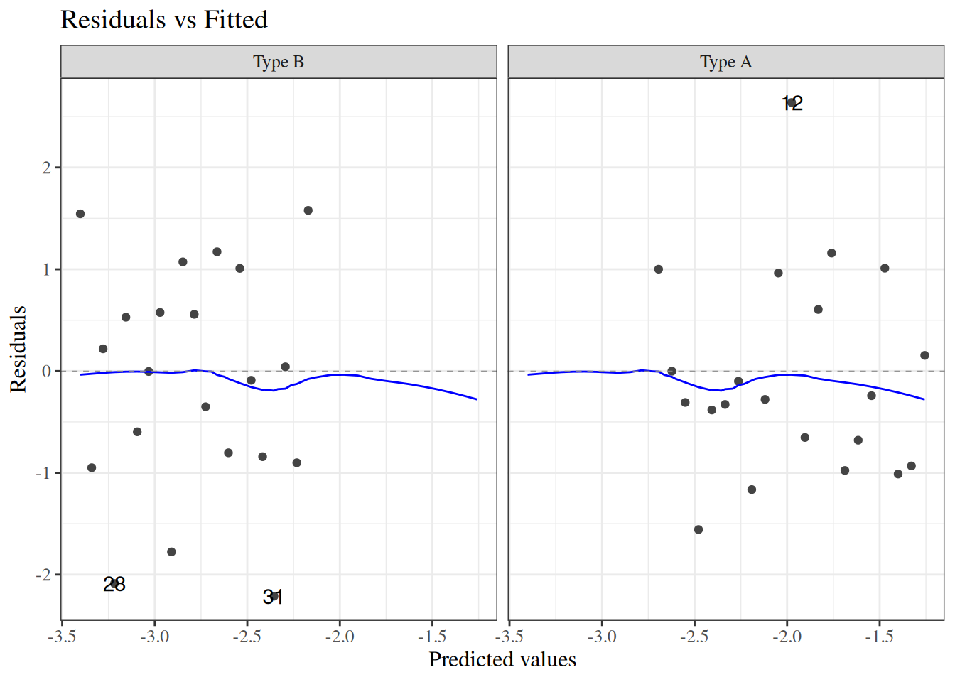
Don’t worry about these options for now; I chose them to match autoplot() as closely as I can. plot.glm and autoplot use stats::lowess instead of stats::loess; stats::lowess is older, hard to use with geom_smooth, and hard to match exactly with stats::loess; see https://support.bioconductor.org/p/2323/.]

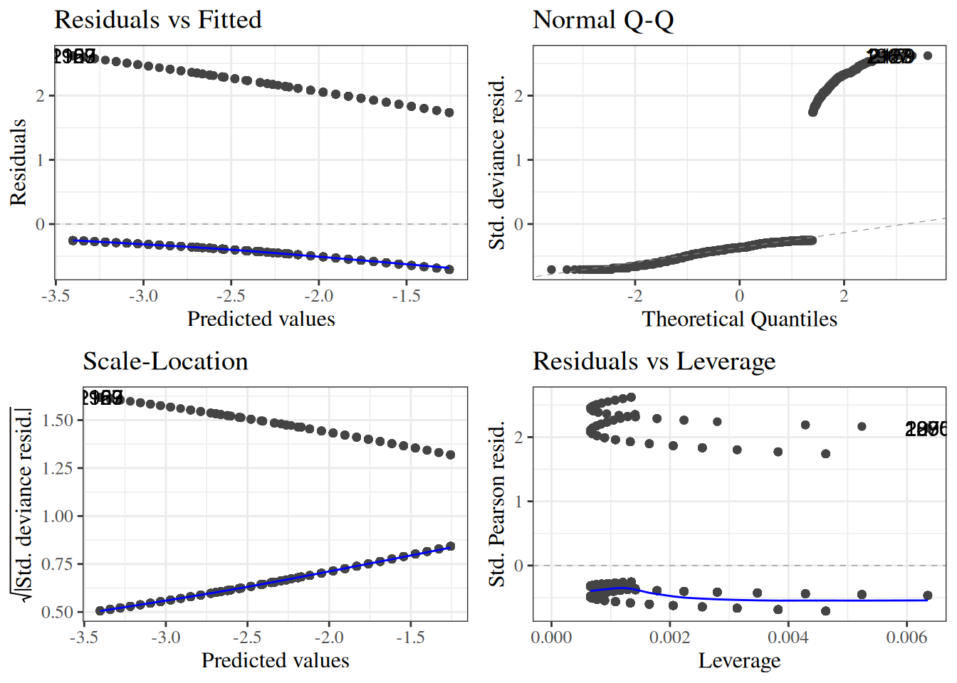
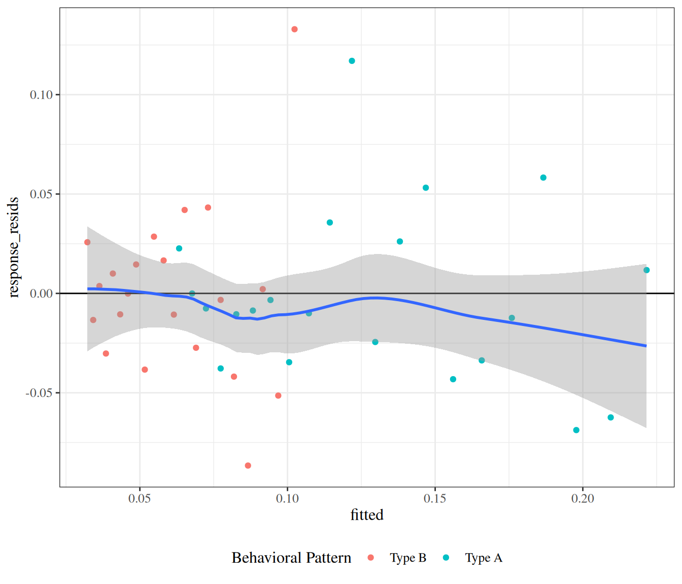
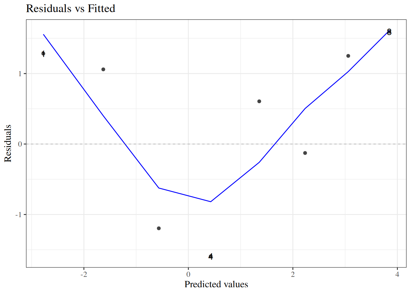
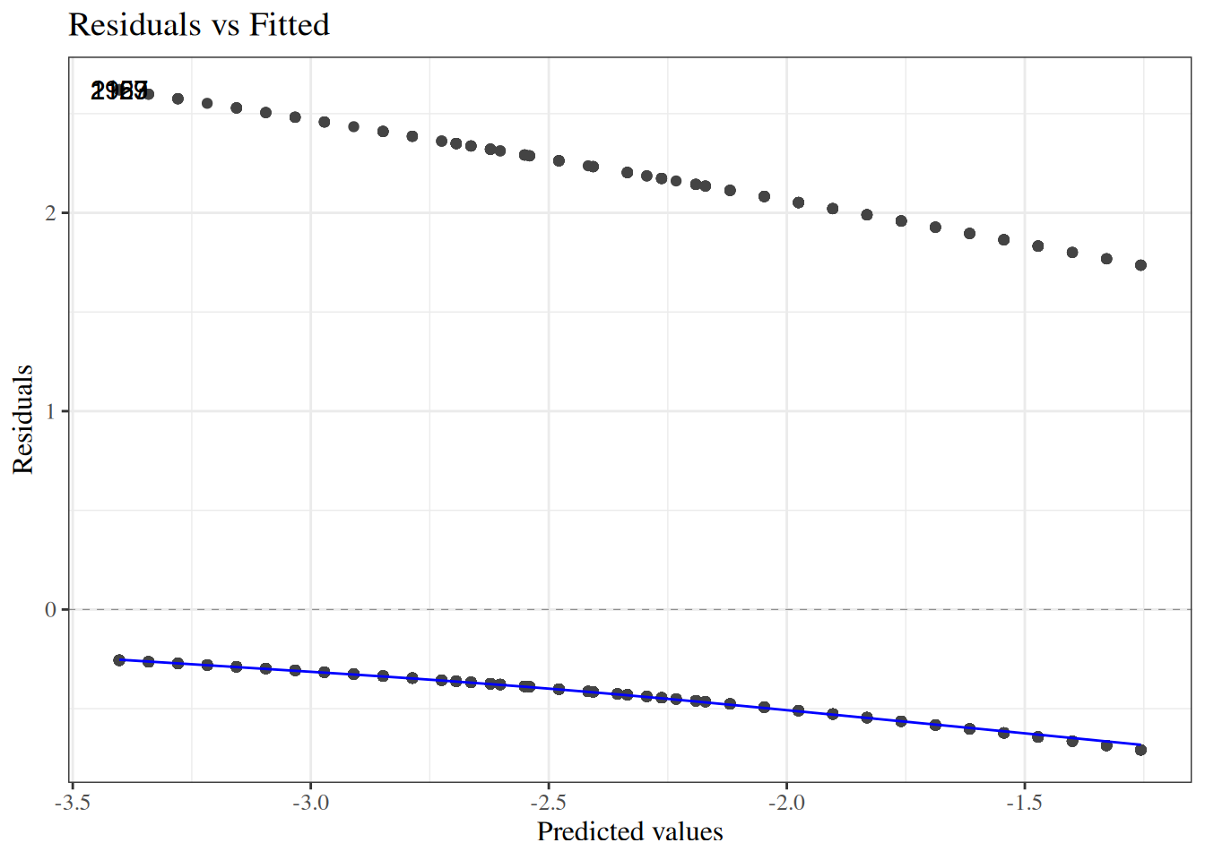
wcgs_response_resid_plot |> print()

Figure 23: residuals plot for wcgs model

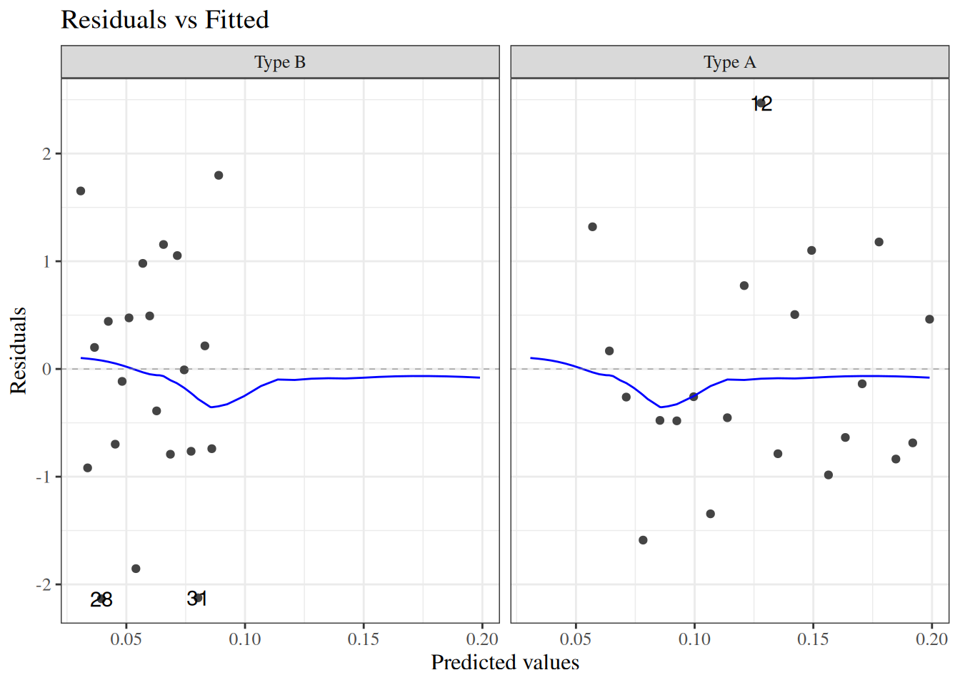
We can see a slight fan-shape here: observations on the right have larger variance (as expected since \(var(\bar y) = \pi(1-\pi)/n\) is maximized when \(\pi = 0.5\)).

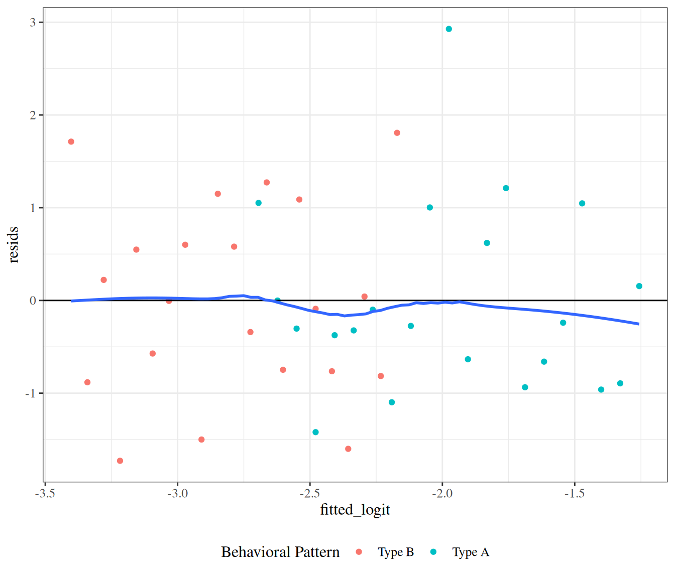
Pearson residuals

The fan-shape in the response residuals plot isn’t necessarily a concern here, since we haven’t made an assumption of constant residual variance, as we did for linear regression.

However, we might want to divide by the standard error in order to make the graph easier to interpret. Here’s one way to do that:

The Pearson (chi-squared) residual for covariate pattern \(k\) is: \[ \begin{aligned} X_k &= \frac{\bar y_k - \hat\pi_k}{\sqrt{\hat \pi_k (1-\hat\pi_k)/n_k}} \end{aligned} \]

where \[ \begin{aligned} \hat\pi_k &\stackrel{\text{def}}{=}\hat\pi(x_k)\\ &\stackrel{\text{def}}{=}\hat P(Y=1|X=x_k)\\ &\stackrel{\text{def}}{=}\text{expit}(x_i'\hat \beta)\\ &\stackrel{\text{def}}{=}\text{expit}(\hat \beta_0 + \sum_{j=1}^p \hat \beta_j x_{ij}) \end{aligned} \]

Let’s take a look at the Pearson residuals for our CHD model from the WCGS data (graphed against the fitted values on the logit scale):

library(ggfortify)

autoplot(chd_glm_contrasts_grouped, which = 1, ncol = 1) |> print()

The fan-shape is gone, and these residuals don’t show any obvious signs of model fit issues.

Pearson residuals plot for beetles data

If we create the same plot for the beetles model, we see some strong evidence of a lack of fit:

library(glmx)
library(dplyr)
data(BeetleMortality)
beetles <- BeetleMortality |>
  mutate(
    pct = died / n,
    survived = n - died,
    dose_c = dose - mean(dose)
  )
beetles_glm_grouped <- beetles |>
  glm(
    formula = cbind(died, survived) ~ dose,
    family = "binomial"
  )
autoplot(beetles_glm_grouped, which = 1, ncol = 1) |> print()

Pearson residuals with individual (ungrouped) data

What happens if we try to compute residuals without grouping the data by covariate pattern?

library(ggfortify)

chd_glm_strat <- glm(
  "formula" = chd69 == "Yes" ~ dibpat + dibpat:age - 1,
  "data" = wcgs,
  "family" = binomial(link = "logit")
)

autoplot(chd_glm_strat, which = 1, ncol = 1) |> print()

Meaningless.

Residuals plot by hand (optional section)

If you want to check your understanding of what these residual plots are, try building them yourself:

wcgs_grouped <-
  wcgs_grouped |>
  mutate(
    fitted = chd_glm_contrasts_grouped |> fitted(),
    fitted_logit = fitted |> logit(),
    resids = chd_glm_contrasts_grouped |> resid(type = "pearson")
  )

wcgs_resid_plot1 <-
  wcgs_grouped |>
  ggplot(
    mapping = aes(
      x = fitted_logit,
      y = resids
    )
  ) +
  geom_point(
    aes(col = dibpat)
  ) +
  geom_hline(yintercept = 0) +
  geom_smooth(
    se = FALSE,
    method.args = list(
      span = 2 / 3,
      degree = 1,
      family = "symmetric",
      iterations = 3,
      surface = "direct"
    ),
    method = stats::loess
  )
# plot.glm and autoplot use stats::lowess, which is hard to use with
# geom_smooth and hard to match exactly;
# see https://support.bioconductor.org/p/2323/

wcgs_resid_plot1 |> print()

Pearson chi-squared goodness of fit test

The Pearson chi-squared goodness of fit statistic is: \[X^2 = \sum_{k=1}^m X_k^2\]

Under the null hypothesis that the model in question is correct (i.e., sufficiently complex), \(X^2\ \dot \sim\ \chi^2(N-p)\).

x_pearson <- chd_glm_contrasts_grouped |>
  resid(type = "pearson")

chisq_stat <- sum(x_pearson^2)

pval <- pchisq(
  chisq_stat,
  lower = FALSE,
  df = length(x_pearson) - length(coef(chd_glm_contrasts_grouped))
)

For our CHD model, the p-value for this test is 0.265236; no significant evidence of a lack of fit at the 0.05 level.

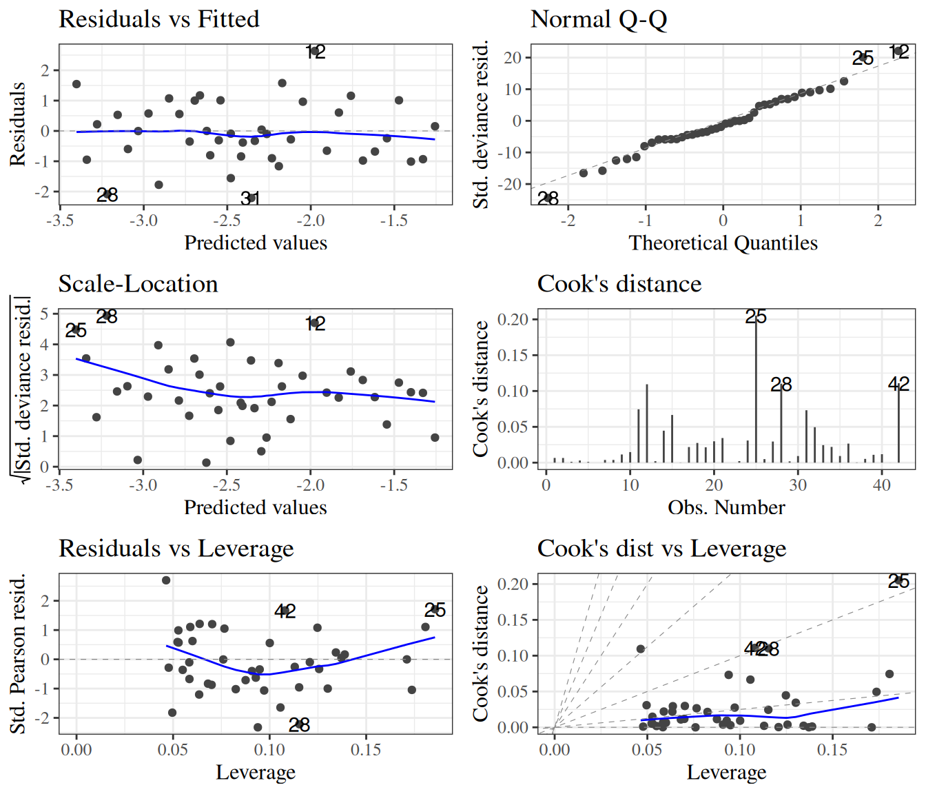
Standardized Pearson residuals

Especially for small data sets, we might want to adjust our residuals for leverage (since outliers in \(X\) add extra variance to the residuals):

\[r_{P_k} = \frac{X_k}{\sqrt{1-h_k}}\]

where \(h_k\) is the leverage of \(X_k\). The functions autoplot() and plot.lm() use these for some of their graphs.

Deviance residuals

For large sample sizes, the Pearson and deviance residuals will be approximately the same. For small sample sizes, the deviance residuals from covariate patterns with small sample sizes can be unreliable (high variance).

\[d_k = \text{sign}(y_k - n_k \hat \pi_k)\left\{\sqrt{2[\ell_{\text{full}}(x_k) - \ell(\hat\beta; x_k)]}\right\}\]

Standardized deviance residuals

\[r_{D_k} = \frac{d_k}{\sqrt{1-h_k}}\]

Diagnostic plots

Let’s take a look at the full set of autoplot() diagnostics now for our CHD model:

chd_glm_contrasts_grouped |>
  autoplot(which = 1:6) |>
  print()

Figure 24: Diagnostics for CHD model

Things look pretty good here. The QQ plot is still usable; with large samples; the residuals should be approximately Gaussian.

Beetles

Let’s look at the beetles model diagnostic plots for comparison:

beetles_glm_grouped |>
  autoplot(which = 1:6) |>
  print()

Figure 25: Diagnostics for logistic model of BeetleMortality data

Hard to tell much from so little data, but there might be some issues here.

10 Alternatives to reporting odds ratios

Objections to odds ratios

Some scholars have raised objections to the use of odds ratios as an effect measurement (Sackett et al. 1996; Norton et al. 2024).

As we saw in Figure 3, the odds ratio is not very closely correlated with the risk difference, and the risk difference is typically the metric that ultimately matters for policy decisions.

Another objection is that odds ratios (and risk ratios, and risk differences) depend on the set of covariates in a logistic regression model, even when those covariates are independent of the exposure of interest and do not interact with that exposure. For example, consider the following model:

\[\text{P}(Y=y|X=x,C=c) = {\color{red}\pi(x,c)}^y (1-{\color{red}\pi(x,c)})^{1-y}\]

\[{\color{red}\pi(x,c)} = \text{expit}{\left\{\eta_0 + \beta_Xx + \beta_Cc\right\}}\]

Then:

\[ \begin{aligned} \text{E}{\left[Y|X=x\right]} &= \text{E}{\left[\text{E}{\left[Y | X, C\right]} | X=x\right]} \\ &= \text{E}{\left[\pi(X,C) | X=x\right]} \\ &= \text{E}{\left[\text{expit}{\left\{\eta_0 + \beta_X X + \beta_C C\right\}} | X=x\right]} \\ &= \int_c{\text{expit}{\left\{\eta_0 + \beta_X x + \beta_C c\right\}} ~\text{p}(C=c|X=x)~ \partial c} \\ &= \int_c{\pi(x,c)~ \text{p}(C=c|X=x)~ \partial c} \end{aligned} \]

Since the \(\text{expit}{\left\{\right\}}\) function is nonlinear, we can’t change the order of the expectation and \(\text{expit}{\left\{\right\}}\) operators:

\[\text{E}{\left[\text{expit}{\left\{\eta_0 + \beta_XX + \beta_CC\right\}} | X\right]} \neq \text{expit}{\left\{\text{E}{\left[\eta_0 + \beta_XX + \beta_CC\right]} | X\right\}}\]

In contrast, consider a model with an identity link function:

\[\text{P}(Y=y|X=x,C=c) = {\color{red}\pi(x,c)}^y (1-{\color{red}\pi(x,c)})^{1-y}\]

\[{\color{red}\pi(x,c)} = \eta_0 + \beta_Xx + \beta_Cc\]

Then:

\[ \begin{aligned} \text{E}{\left[Y|X=x\right]} &= \text{E}{\left[\text{E}{\left[Y | X, C\right]} | X=x\right]} \\ &= \text{E}{\left[\eta_0 + \beta_X X + \beta_C C | X=x\right]} \\ &= \text{E}{\left[\eta_0 | X=x\right]} + \text{E}{\left[\beta_X X | X=x\right]} + \text{E}{\left[\beta_C C | X=x\right]} \\ &= {\color{red}\eta_0} + {\color{blue}\beta_X x} + {\color{red} \beta_C\text{E}{\left[ C | X=x\right]}} \\ &= {\color{red}(\eta_0 + \beta_C \text{E}{\left[C|X=x\right]})} + {\color{blue}\beta_Xx} \end{aligned} \]

If \(C \perp\!\!\!\perp X\), then \(\text{E}{\left[C|X=x\right]} = \text{E}{\left[C\right]}\), and we can simplify further:

\[ \begin{aligned} \text{E}{\left[Y|X=x\right]} &= {\color{red}(\eta_0 + \beta_C \text{E}{\left[C|X=x\right]})} + {\color{blue}\beta_Xx} \\ &= {\color{red}(\eta_0 + \beta_C \text{E}{\left[C\right]})} + {\color{blue}\beta_Xx} \\&= {\color{red}\eta_0^*} + {\color{blue}\beta_Xx} \end{aligned} \]

Then:

\[ \begin{aligned} \frac{\partial}{\partial x} \text{E}{\left[Y|X=x\right]} = {\color{blue}\beta_X} = \frac{\partial}{\partial x} \text{E}{\left[Y|X=x,C=c\right]} \end{aligned} \]

In other words, for a model with an identity link function, if covariates \(X\) and \(C\) are independent, then the slope with respect to \(X\) doesn’t depend on whether \(C\) is included in the model (and an analogous result holds if \(X\) is discrete or categorical).

Exercise 48 What are the expressions for \(\text{E}{\left[Y|X=x\right]}\) and \(\frac{\partial}{\partial x} \text{E}{\left[Y|X=x\right]}\) for the model above, if \(\text{E}{\left[C|X=x\right]} = \gamma_0 + \gamma_x x\)?

Solution 41. Left to the reader.

Exercise 49 What are the expressions for \(\text{E}{\left[Y|X=x\right]}\) and \(\frac{\partial}{\partial x} \text{E}{\left[Y|X=x\right]}\), if instead of the model above, \[\pi(x,c) = \eta_0 + \beta_Xx + \beta_Cc +\beta_{XC}xc\] and \(\text{E}{\left[C|X=x\right]} = \gamma_0 + \gamma_x x\)?

Solution 42. Left to the reader.

Hint: does adding the interaction term change the functional form of \(\text{E}{\left[Y|X=x\right]}\)?

Deriving risk ratios and risk differences from logistic regression models

If you want to report risk differences or risk ratios instead of odds ratios, you can obtain estimates from logistic regression models, as long as you didn’t stratify sampling by the outcome; in other words, not in case-control studies (see Section 1.3.3.4).

To compute risk ratios from logistic regression models:

• Apply the expit function to the linear predictor for each covariate pattern to compute the (estimated) risks,
• Then take the differences or ratios of the risks, as needed.

To quantify uncertainty for risk difference or risk ratio estimates derived from logistic regression models (e.g., to calculate SEs, CIs, and p-values), you will need to use the bootstrap, the multivariate delta method, or some other special technique.

Other link functions for Bernoulli outcomes

Alternatively, if you want to estimate risk ratios more directly from the model, you can sometimes change the link function from \(\text{logit}{\left\{\right\}}\) to \(\text{log}{\left\{\right\}}\); then you can obtain risk ratios by exponentiating coefficients ¹, just like we did for odds ratios with the logit link:

data(anthers, package = "dobson")
anthers_sum <- aggregate(
  anthers[c("n", "y")],
  by = anthers[c("storage")], FUN = sum
)

anthers_glm_log <- glm(
  formula = cbind(y, n - y) ~ storage,
  data = anthers_sum,
  family = binomial(link = "log")
)

anthers_glm_log |>
  parameters() |>
  print_md()

Parameter	Log-Risk	SE	95% CI	z	p
(Intercept)	-0.80	0.12	(-1.04, -0.58)	-6.81	< .001
storage	0.17	0.07	(0.02, 0.31)	2.31	0.021

1. or linear combinations of coefficients, depending on what covariate patterns you are contrasting

Now \(\text{exp}{\left\{\beta\right\}}\) gives us risk ratios instead of odds ratios:

anthers_glm_log |>
  parameters(exponentiate = TRUE) |>
  print_md()

Parameter	Risk Ratio	SE	95% CI	z	p
(Intercept)	0.45	0.05	(0.35, 0.56)	-6.81	< .001
storage	1.18	0.09	(1.03, 1.36)	2.31	0.021

Let’s compare this model with a logistic model:

anthers_glm_logit <- glm(
  formula = cbind(y, n - y) ~ storage,
  data = anthers_sum,
  family = binomial(link = "logit")
)

anthers_glm_logit |>
  parameters(exponentiate = TRUE) |>
  print_md()

Parameter	Odds Ratio	SE	95% CI	z	p
(Intercept)	0.76	0.20	(0.45, 1.27)	-1.05	0.296
storage	1.49	0.26	(1.06, 2.10)	2.29	0.022

[to add: fitted plots on each outcome scale]

When I try to use link ="log" in practice, I often get errors about not finding good starting values for the estimation procedure. This is likely because the model is producing fitted probabilities greater than 1.

When this happens, you can try to fit Poisson regression models instead (we will see those soon!). But then the outcome distribution isn’t quite right, and you won’t get warnings about fitted probabilities greater than 1. In my opinion, the Poisson model for binary outcomes is confusing and not very appealing.

WCGS: link functions

wcgs_glm_logit_link <- chd_grouped_data |>
  mutate(type = relevel(dibpat, ref = "Type B")) |>
  glm(
    "formula" = cbind(x, `n - x`) ~ dibpat * age,
    "data" = _,
    "family" = binomial(link = "logit")
  )

wcgs_glm_identity_link <-
  chd_grouped_data |>
  mutate(type = relevel(dibpat, ref = "Type B")) |>
  glm(
    "formula" = cbind(x, `n - x`) ~ dibpat * age,
    "data" = _,
    "family" = binomial(link = "identity")
  )
wcgs_glm_identity_link |>
  coef() |>
  pander()

(Intercept)	dibpatType A	age	dibpatType A:age
-0.08257	-0.1374	0.002906	0.004194

library(ggfortify)
wcgs_glm_logit_link |> autoplot(which = c(1), ncol = 1) + facet_wrap(~dibpat)
wcgs_glm_identity_link |> autoplot(which = c(1), ncol = 1) + facet_wrap(~dibpat)

Figure 26: Residuals vs Fitted plot for wcgs models

(a) Logistic link

(b) Identity link

beetles_lm <-
  beetles_long |>
  lm(formula = died ~ dose)

beetles_glm_grouped <- beetles |>
  glm(formula = cbind(died, survived) ~ dose, family = "binomial")


beetles <-
  beetles |> mutate(
    resid_logit = beetles_glm_grouped |> resid(type = "response")
  )
beetles_glm_grouped |> autoplot(which = c(1), ncol = 1)
beetles_lm |> autoplot(which = c(1), ncol = 1)

Figure 27: Residuals vs Fitted plot for BeetleMortality models

(a) Logistic link

(b) Identity link

Quasibinomial

See Hua Zhou’s lecture notes

11 Further reading

• Hosmer et al. (2013) is a classic textbook on logistic regression

Bliss, C. I. 1935. “The Calculation of the Dosage-Mortality Curve.” Annals of Applied Biology 22 (1): 134–67. https://doi.org/10.1111/j.1744-7348.1935.tb07713.x.

Dobson, Annette J, and Adrian G Barnett. 2018. An Introduction to Generalized Linear Models. 4th ed. CRC press. https://doi.org/10.1201/9781315182780.

Hosmer, David W, Stanley Lemeshow, and Rodney X Sturdivant. 2013. Applied Logistic Regression. John Wiley & Sons. https://onlinelibrary.wiley.com/doi/book/10.1002/9781118548387.

Lee, James. 1994. “Odds Ratio or Relative Risk for Cross-Sectional Data?” International Journal of Epidemiology (England) 23 (1): 201–3. https://doi.org/10.1093/ije/23.1.201.

Lumley, Thomas. 2010. Complex Surveys : A Guide to Analysis Using R. Wiley Series in Survey Methodology. John Wiley. https://doi.org/10.1002/9780470580066.

Nahhas, Ramzi W. 2024. Introduction to Regression Methods for Public Health Using R. CRC Press. https://www.bookdown.org/rwnahhas/RMPH/.

Norton, Edward C., Bryan E. Dowd, Melissa M. Garrido, and Matthew L. Maciejewski. 2024. “Requiem for Odds Ratios.” Health Services Research 59 (4): e14337. https://doi.org/https://doi.org/10.1111/1475-6773.14337.

Rosenman, Ray H, Richard J Brand, C David Jenkins, Meyer Friedman, Reuben Straus, and Moses Wurm. 1975. “Coronary Heart Disease in the Western Collaborative Group Study: Final Follow-up Experience of 8 1/2 Years.” JAMA 233 (8): 872–77. https://doi.org/10.1001/jama.1975.03260080034016.

Sackett, David L, Jonathan J Deeks, and Doughs G Altman. 1996. “Down with Odds Ratios!” BMJ Evidence-Based Medicine 1 (6): 164.

Vittinghoff, Eric, David V Glidden, Stephen C Shiboski, and Charles E McCulloch. 2012. Regression Methods in Biostatistics: Linear, Logistic, Survival, and Repeated Measures Models. 2nd ed. Springer. https://doi.org/10.1007/978-1-4614-1353-0.