Models for Count Outcomes

Poisson regression and variations

Acknowledgements

This content is adapted from:

• Dobson and Barnett (2018), Chapter 9
• Vittinghoff et al. (2012), Chapter 8

Configuring R

Functions from these packages will be used throughout this document:

library(conflicted) # check for conflicting function definitions
# library(printr) # inserts help-file output into markdown output
library(rmarkdown) # Convert R Markdown documents into a variety of formats.
library(pander) # format tables for markdown
library(ggplot2) # graphics
library(ggfortify) # help with graphics
library(dplyr) # manipulate data
library(tibble) # `tibble`s extend `data.frame`s
library(magrittr) # `%>%` and other additional piping tools
library(haven) # import Stata files
library(knitr) # format R output for markdown
library(tidyr) # Tools to help to create tidy data
library(plotly) # interactive graphics
library(dobson) # datasets from Dobson and Barnett 2018
library(parameters) # format model output tables for markdown
library(haven) # import Stata files
library(latex2exp) # use LaTeX in R code (for figures and tables)
library(fs) # filesystem path manipulations
library(survival) # survival analysis
library(survminer) # survival analysis graphics
library(KMsurv) # datasets from Klein and Moeschberger
library(parameters) # format model output tables for
library(webshot2) # convert interactive content to static for pdf
library(forcats) # functions for categorical variables ("factors")
library(stringr) # functions for dealing with strings
library(lubridate) # functions for dealing with dates and times

Here are some R settings I use in this document:

rm(list = ls()) # delete any data that's already loaded into R

conflicts_prefer(dplyr::filter)
ggplot2::theme_set(
  ggplot2::theme_bw() + 
        # ggplot2::labs(col = "") +
    ggplot2::theme(
      legend.position = "bottom",
      text = ggplot2::element_text(size = 12, family = "serif")))

knitr::opts_chunk$set(message = FALSE)
options('digits' = 6)

panderOptions("big.mark", ",")
pander::panderOptions("table.emphasize.rownames", FALSE)
pander::panderOptions("table.split.table", Inf)
conflicts_prefer(dplyr::filter) # use the `filter()` function from dplyr() by default
legend_text_size = 9
run_graphs = TRUE

1 Introduction

This chapter presents models for count data outcomes. With covariates, the event rate \(\lambda\) becomes a function of the covariates \(\tilde{X}= (X_1, \dots,X_n)\). Typically, count data models use a \(\text{log}{\left\{\right\}}\) link function, and thus an \(\text{exp}{\left\{\right\}}\) inverse-link function. That is:

\[ \begin{aligned} \text{E}[Y | \tilde{X}= \tilde{x}, T = t] &= \mu(\tilde{x},t) \\ \mu(\tilde{x},t) &= \lambda(\tilde{x})\cdot t \\ \lambda(\tilde{x}) &= \text{exp}{\left\{\eta(\tilde{x})\right\}} \\ \eta(\tilde{x}) &= \tilde{x}'\tilde \beta = \beta_0 + \beta_1 x_1 + \dots + \beta_p x_p \end{aligned} \tag{1}\]

\(T=t\) is called the exposure magnitude and has a special role in this model.

Exercise 1 Where have we seen a relationship like \[\mu = \lambda \cdot t\] before?

Solution 1. The relationship \[\mu = \lambda \cdot t\] in count regression models is analogous to the relationship \[\mu = n \pi\] in Binomial models.

We can also think of \(t\) as a special part of the linear component:

\[ \begin{aligned} \text{log}{\left\{\text{E}[Y | \tilde{X}= \tilde{x},T=t]\right\}} &= \text{log}{\left\{\mu(\tilde{x})\right\}}\\ &=\text{log}{\left\{\lambda(\tilde{x}) \cdot t\right\}}\\ &=\text{log}{\left\{\lambda(\tilde{x})\right\}} + \log{t}\\ &=\text{log}{\left\{\text{exp}{\left\{\eta(\tilde{x})\right\}}\right\}} + \log{t}\\ &=\eta(\tilde{x}) + \log{t}\\ &=\tilde{x}'\tilde\beta + \log{t}\\ &=(\beta_0 +\beta_1 x_1+\dots + \beta_p x_p) + \log{t}\\ \end{aligned} \]

In contrast with the other covariates (represented by \(\tilde{X}\)), \(t\) enters this expression with a \(\log{}\) transformation and without a corresponding \(\beta\) coefficient; in other words, \(\text{log}{\left\{t\right\}}\) is an offset term.

Exercise 2 What are the units of \(\mu\) in Equation 1?

Solution 2. \(\mu\) is the mean of \(Y\), and \(Y\) is a count, so \(\mu\) is also a count; for example:

• 3.1 cyclones,
• 10.23 ER visits
• 15.01 infections

Exercise 3 What are the units of \(\lambda\) in Equation 1?

Solution 3. \(\lambda = \mu/t\), so \(\lambda\) is a rate of counts per unit of \(t\). For example:

• 3.1 cyclones per year
• 2.023 ER visits per 10 person-years
• 15.01 infections per 1000 person-years at risk

2 Interpreting Poisson regression models

Differences on the log-rate scale become ratios on the rate scale, because

\[\text{exp}{\left\{a-b\right\}} = \frac{\text{exp}{\left\{a\right\}}}{\text{exp}{\left\{b\right\}}}\]

(recall from Algebra 2)

Therefore, according to this model, differences of \(\delta\) in covariate \(x_j\) correspond to rate ratios of \(\text{exp}{\left\{\beta_j \cdot \delta\right\}}\).

That is, letting \(\tilde{X}_{-j}\) denote vector \(\tilde{X}\) with element \(j\) removed:

\[ \begin{aligned} &{ \left\{ \log{\text{E}[Y |{\color{red}{X_j = a}}, \tilde{X}_{-j}=\tilde{x}_{-j},T=t]} \atop {-\log{\text{E}[Y |{\color{red}{X_j = b}}, \tilde{X}_{-j}=\tilde{x}_{-j},T=t]}} \right\} }\\ &= {\left\{ \log{t} + \beta_0 + \beta_1 x_1 + ... + {\color{red}{\beta_j (a)}} + ...+\beta_p x_p \atop {-\log{t} + \beta_0 + \beta_1 x_1 + ... + {\color{red}{\beta_j (b)}} + ...+\beta_p x_p} \right\}}\\ &= \color{red}{\beta_j(a-b)} \end{aligned} \]

And accordingly,

\[ \begin{aligned} \frac {\mathbb{E}[Y |{\color{red}{X_j = a}}, \tilde{X}_{-j} = \tilde{x}_{-j}, T = t] } { \text{E}[Y |{\color{red}{X_j = b}}, \tilde{X}_{-j}=\tilde{x}_{-j},T=t] } = \text{exp}{\left\{{\color{red}{\beta_j(a-b)}}\right\}} \end{aligned} \]

3 Example: needle-sharing

(adapted from Vittinghoff et al. (2012), §8)

library(tidyverse)
library(haven)
needles = 
  "inst/extdata/needle_sharing.dta" |> 
  read_dta() |>
  as_tibble() |>
  mutate(
    hivstat =
      hivstat |>
      case_match(
        1 ~ "HIV+",
        0 ~ "HIV-") |> 
      factor() |> 
      relevel(ref = "HIV-"),
    polydrug =
      polydrug |>
      case_match(
        1 ~ "multiple drugs used",
        0 ~ "one drug used") |>
      factor() |>
      relevel(ref = "one drug used"),
    homeless = 
      homeless |> 
      case_match(
        1 ~ "homeless", 
        0 ~ "not homeless") |>
      factor() |>
      relevel(ref = "not homeless"),
    ethn = ethn |> factor() |> relevel(ref = "White"),
    sex = sex |> factor() |> relevel(ref = "M")
  ) |> 
  labelled::set_variable_labels(
    "sex" = "sex (reference = Male)",
    "ethn" = "ethnicity (reference = White)",
    "shsyryn"  = "shared syringe yes/no (1 = yes, 0 = no)",
    "logshsyr" = "log(No. of shared needles)",
    "polydrug" = "how many drugs used?",
    "sqrtninj" = "sqrt(No. of infections in 30 days)",
    "homeless" = "Homeless (1 = yes, 0 = no)",
    "hivstat" = "HIV status (reference = HIV-)"
  )

dict <- tibble(
  variable = names(needles),
  description = labelled::get_variable_labels(needles) |> 
    sapply(function(x) ifelse(is.null(x), "", x)),
)
dict |> pander::pander()

Table 1: Data dictionary for needles data

variable	description
id	ID
sex	sex (reference = Male)
ethn	ethnicity (reference = White)
age	Age at 1st interview
dprsn_dx	DPRSN_DX
sexabuse	Sexually abused?
shared_syr	Shared syringe
hivstat	HIV status (reference = HIV-)
hplsns	HPLSNS
nivdu	No of injections (in 30 days)
shsyryn	shared syringe yes/no (1 = yes, 0 = no)
sqrtnivd	sqrt(No ivdu 30 days)
logshsyr	log(No. of shared needles)
polydrug	how many drugs used?
sqrtninj	sqrt(No. of infections in 30 days)
homeless	Homeless (1 = yes, 0 = no)
shsyr	No. of shared needles

needles

Table 2: Needle-sharing data

library(ggplot2)

needles |> 
  ggplot(
    aes(
      x = age,
      y = shsyryn,
      shape = sex,
      col = ethn
    )
  ) + 
  geom_point(
    aes(size = nivdu), 
    alpha = .5) +
  scale_size_area(max_size = 4) +
  facet_grid(
    cols = vars(polydrug), 
    rows = vars(homeless)) +
  theme(legend.position = "bottom")

Figure 1: Rates of needle sharing

Covariate counts

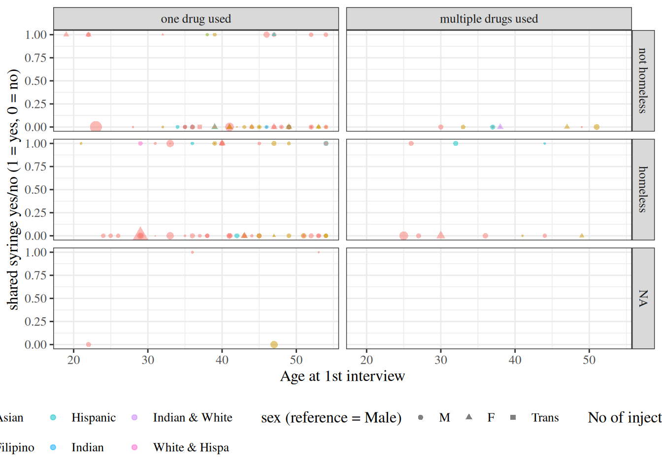
Table 3: Counts of observations in needles dataset by sex, unhoused status, and multiple drug use

needles |> 
  dplyr::select(sex, homeless, polydrug) |> 
  summary()
#>     sex             homeless                 polydrug  
#>  M    :97   not homeless:63   one drug used      :109  
#>  F    :30   homeless    :61   multiple drugs used: 19  
#>  Trans: 1   NA's        : 4

There’s only one individual with sex = Trans, which unfortunately isn’t enough data to analyze. We will remove that individual:

needles = needles |> filter(sex != "Trans")

Model

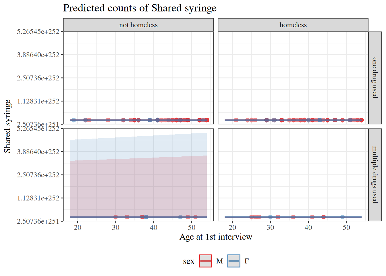
glm1 = 
  needles |> 
  dplyr::filter(nivdu > 0) |> 
  glm(
    offset = log(nivdu),
    family = stats::poisson,
    formula = shared_syr ~ age + sex + homeless*polydrug
  )
library(equatiomatic)
equatiomatic::extract_eq(glm1)

\[ \log ({ E( \operatorname{shared_syr} ) }) = \alpha + \beta_{1}(\operatorname{age}) + \beta_{2}(\operatorname{sex}_{\operatorname{F}}) + \beta_{3}(\operatorname{homeless}) + \beta_{4}(\operatorname{polydrug}) + \beta_{5}(\operatorname{homeless} \times \operatorname{polydrug}) + \operatorname{(offset)} \]

library(parameters)
glm1 |> parameters(exponentiate = TRUE) |> 
  print_md()

Table 4: Poisson model for needle-sharing data

Parameter	IRR	SE	95% CI	z	p
(Intercept)	0.02	4.02e-03	(9.09e-03, 0.03)	-15.87	< .001
age	1.00	5.85e-03	(0.99, 1.01)	0.42	0.673
sex (F)	1.37	0.16	(1.09, 1.72)	2.73	0.006
homeless (homeless)	2.77	0.34	(2.18, 3.53)	8.30	< .001
polydrug (multiple drugs used)	2.85e-07	8.71e-05	(1.59e-267, 5.11e+253)	-0.05	0.961
homeless (homeless) × polydrug (multiple drugs used)	6.21e+05	1.90e+08	(3.47e-255, 1.11e+266)	0.04	0.965

library(sjPlot)
glm1 |> 
  sjPlot::plot_model(
    type = "pred",
    terms = c("age", "sex", "homeless", "polydrug"),
    show.data = TRUE
  ) +
  theme(legend.position = "bottom")

Figure 2

4 Inference for count regression models

Confidence intervals for regression coefficients and rate ratios

As usual:

\[ \beta \in \left[\hat \beta{\color{red}\pm} z_{1 - \frac{\alpha}{2}}\cdot \widehat{\text{se}}{\left(\hat \beta\right)}\right] \]

Rate ratios: exponentiate CI endpoints

\[ \text{exp}{\left\{\beta\right\}} \in \left[\text{exp}{\left\{\hat \beta{\color{red}\pm} z_{1 - \frac{\alpha}{2}}\cdot \widehat{\text{se}}{\left(\hat \beta\right)}\right\}} \right] \]

Hypothesis tests for regression coefficients

\[ z = \frac{\hat \beta - \beta_0}{\widehat{\text{se}}{\left(\hat \beta\right)}} \]

Compare \(z\) or \(|z|\) to the tails of the standard Gaussian distribution, according to the null hypothesis.

Comparing nested models

log(likelihood ratio) tests, as usual.

5 Prediction

\[ \begin{aligned} \hat y &\stackrel{\text{def}}{=}\hat{\text{E}}[Y|\tilde{X}= \tilde{x},T=t]\\ &=\hat\mu(\tilde{x}, t)\\ &=\hat\lambda(\tilde{x}) \cdot t\\ &=\text{exp}{\left\{\hat\eta(\tilde{x})\right\}} \cdot t\\ &=\text{exp}{\left\{\tilde{x}'\hat{\tilde{\beta}}\right\}} \cdot t \end{aligned} \]

6 Diagnostics

Residuals

Observation residuals

\[e \stackrel{\text{def}}{=}y - \hat y\]

Pearson residuals

\[r = \frac{e}{\widehat{\text{se}}{\left(e\right)}} \approx \frac{e}{\sqrt{\hat y}}\]

Standardized Pearson residuals

\[r_p = \frac{r}{\sqrt{1-h}}\] where \(h\) is the “leverage” (which we will continue to leave undefined).

Deviance residuals

\[ d_k = \text{sign}(y - \hat y)\left\{\sqrt{2[\ell_{\text{full}}(y) - \ell(\hat\beta; y)]}\right\} \]

Note

\[\text{sign}(x) \stackrel{\text{def}}{=}\frac{x}{|x|}\] In other words:

• \(\text{sign}(x) = -1\) if \(x < 0\)
• \(\text{sign}(x) = 0\) if \(x = 0\)
• \(\text{sign}(x) = 1\) if \(x > 0\)

library(ggfortify)
autoplot(glm1)

Table 5: Diagnostics for Poisson model

7 Zero-inflation

Models for zero-inflated counts

We assume a latent (unobserved) binary variable, \(Z\), which we model using logistic regression:

\[P(Z=1|X=x) = \pi(x) = \text{expit}(\gamma_0 + \gamma_1 x_1 +...)\]

According to this model, if \(Z=1\), then \(Y\) will always be zero, regardless of \(X\) and \(T\):

\[P(Y=0|Z=1,X=x,T=t) = 1\]

Otherwise (if \(Z=0\)), \(Y\) will have a Poisson distribution, conditional on \(X\) and \(T\), as above.

Even though we never observe \(Z\), we can estimate the parameters \(\gamma_0\)-\(\gamma_p\), via maximum likelihood:

\[ \begin{aligned} \text{P}(Y=y|X=x,T=t) &= \text{P}(Y=y,Z=1|...) + \text{P}(Y=y,Z=0|...) \end{aligned} \] (by the Law of Total Probability)

where \[ \begin{aligned} P(Y=y,Z=z|...) &= P(Y=y|Z=z,...)P(Z=z|...) \end{aligned} \]

Exercise 4 Expand \(P(Y=0|X=x,T=t)\), \(P(Y=1|X=x,T=t)\) and \(P(Y=y|X=x,T=t)\) into expressions involving \(P(Z=1|X=x,T=t)\) and \(P(Y=y|Z=0,X=x,T=t)\).

Exercise 5 Derive the expected value and variance of \(Y\), conditional on \(X\) and \(T\), as functions of \(P(Z=1|X=x,T=t)\) and \(\text{E}[Y|Z=0,X=x,T=t]\).

8 Over-dispersion

The Poisson distribution model forces the variance to equal the mean. In practice, many count distributions will have a variance substantially larger than the mean (or occasionally, smaller).

Definition 1 (Overdispersion) A random variable \(X\) is overdispersed relative to a model \(\text{p}(X=x)\) if if its empirical variance in a dataset is larger than the value is predicted by the fitted model \(\hat{\text{p}}(X=x)\).

c.f. Dobson and Barnett (2018) §3.2.1, 7.7, 9.8; Vittinghoff et al. (2012) §8.1.5; and https://en.wikipedia.org/wiki/Overdispersion.

When we encounter overdispersion, we can try to reduce the residual variance by adding more covariates.

Note

Logistic regression is named after the (inverse) link function. Poisson regression is named after the outcome distribution. I think this naming convention reflects the strongest (most questionable assumption) in the model. In binary data regression, the outcome distribution essentially must be Bernoulli (or Binomial), but the link function could be logit, log, identity, probit, or something more unusual. In count data regression, the outcome distribution could have many different shapes, but the link function will probably end up being log, so that covariates have multiplicative effects on the rate.

8.1 Negative binomial models

There are alternatives to the Poisson model. Most notably, the negative binomial model.

We can still model \(\mu\) as a function of \(X\) and \(T\) as before, and we can combine this model with zero-inflation (as the conditional distribution for the non-zero component).

Example: needle-sharing

library(MASS) #need this for glm.nb()
glm1.nb = glm.nb(
  data = needles,
  shared_syr ~ age + sex + homeless*polydrug
)

equatiomatic::extract_eq(glm1.nb)

\[ \log ({ E( \operatorname{shared_syr} ) }) = \alpha + \beta_{1}(\operatorname{age}) + \beta_{2}(\operatorname{sex}_{\operatorname{F}}) + \beta_{3}(\operatorname{homeless}) + \beta_{4}(\operatorname{polydrug}) + \beta_{5}(\operatorname{homeless} \times \operatorname{polydrug}) \]

Table 6: Negative binomial model for needle-sharing data

summary(glm1.nb)
#> 
#> Call:
#> glm.nb(formula = shared_syr ~ age + sex + homeless * polydrug, 
#>     data = needles, init.theta = 0.08436295825, link = log)
#> 
#> Coefficients:
#>                                               Estimate Std. Error z value
#> (Intercept)                                   9.91e-01   1.71e+00    0.58
#> age                                          -2.76e-02   3.82e-02   -0.72
#> sexF                                          1.06e+00   8.07e-01    1.32
#> homelesshomeless                              1.65e+00   7.22e-01    2.29
#> polydrugmultiple drugs used                  -2.46e+01   3.61e+04    0.00
#> homelesshomeless:polydrugmultiple drugs used  2.32e+01   3.61e+04    0.00
#>                                              Pr(>|z|)  
#> (Intercept)                                     0.563  
#> age                                             0.469  
#> sexF                                            0.187  
#> homelesshomeless                                0.022 *
#> polydrugmultiple drugs used                     0.999  
#> homelesshomeless:polydrugmultiple drugs used    0.999  
#> ---
#> Signif. codes:  0 '***' 0.001 '**' 0.01 '*' 0.05 '.' 0.1 ' ' 1
#> 
#> (Dispersion parameter for Negative Binomial(0.0844) family taken to be 1)
#> 
#>     Null deviance: 69.193  on 119  degrees of freedom
#> Residual deviance: 57.782  on 114  degrees of freedom
#>   (7 observations deleted due to missingness)
#> AIC: 315.5
#> 
#> Number of Fisher Scoring iterations: 1
#> 
#> 
#>               Theta:  0.0844 
#>           Std. Err.:  0.0197 
#> 
#>  2 x log-likelihood:  -301.5060

tibble(name = names(coef(glm1)), poisson = coef(glm1), nb = coef(glm1.nb))

Table 7: Poisson versus Negative Binomial Regression coefficient estimates

zero-inflation

library(glmmTMB)
zinf_fit1 = glmmTMB(
  family = "poisson",
  data  = needles,
  formula = shared_syr ~ age + sex + homeless*polydrug,
  ziformula = ~ age + sex + homeless + polydrug # fit won't converge with interaction
)

zinf_fit1 |>
  parameters(exponentiate = TRUE) |>
  print_md()

Table 8: Zero-inflated poisson model

# Fixed Effects

Parameter	IRR	SE	95% CI	z	p
(Intercept)	3.16	0.82	(1.90, 5.25)	4.44	< .001
age	1.01	5.88e-03	(1.00, 1.02)	1.74	0.081
sex [F]	3.43	0.44	(2.67, 4.40)	9.68	< .001
homeless [homeless]	3.44	0.47	(2.63, 4.50)	9.03	< .001
polydrug [multiple drugs used]	1.85e-09	1.21e-05	(0.00, Inf)	-3.08e-03	0.998
homeless [homeless] × polydrug [multiple drugs used]	1.38e+08	9.04e+11	(0.00, Inf)	2.87e-03	0.998

# Zero-Inflation

Parameter	Odds Ratio	SE	95% CI	z	p
(Intercept)	0.49	0.54	(0.06, 4.25)	-0.65	0.514
age	1.05	0.03	(1.00, 1.10)	1.95	0.051
sex [F]	1.44	0.84	(0.46, 4.50)	0.62	0.533
homeless [homeless]	0.68	0.34	(0.26, 1.80)	-0.78	0.436
polydrug [multiple drugs used]	1.15	0.91	(0.24, 5.43)	0.18	0.858

Another R package for zero-inflated models is pscl (Zeileis et al. (2008)).

zero-inflated negative binomial model

library(glmmTMB)
zinf_fit1 = glmmTMB(
  family = nbinom2,
  data  = needles,
  formula = shared_syr ~ age + sex + homeless*polydrug,
  ziformula = ~ age + sex + homeless + polydrug 
  # fit won't converge with interaction
)

zinf_fit1 |>
  parameters(exponentiate = TRUE) |>
  print_md()

Table 9: Zero-inflated negative binomial model

# Fixed Effects

Parameter	IRR	SE	95% CI	z	p
(Intercept)	1.06	1.48	(0.07, 16.52)	0.04	0.969
age	1.02	0.03	(0.96, 1.08)	0.53	0.599
sex [F]	6.86	6.36	(1.12, 42.16)	2.08	0.038
homeless [homeless]	6.44	4.59	(1.60, 26.01)	2.62	0.009
polydrug [multiple drugs used]	8.25e-10	7.07e-06	(0.00, Inf)	-2.44e-03	0.998
homeless [homeless] × polydrug [multiple drugs used]	2.36e+08	2.02e+12	(0.00, Inf)	2.25e-03	0.998

# Zero-Inflation

Parameter	Odds Ratio	SE	95% CI	z	p
(Intercept)	0.10	0.20	(1.47e-03, 6.14)	-1.11	0.269
age	1.07	0.04	(0.99, 1.15)	1.78	0.075
sex [F]	2.72	2.40	(0.48, 15.33)	1.13	0.258
homeless [homeless]	1.15	0.86	(0.27, 4.96)	0.19	0.853
polydrug [multiple drugs used]	0.75	0.86	(0.08, 7.12)	-0.25	0.799

# Dispersion

Parameter	Coefficient	95% CI
(Intercept)	0.44	(0.11, 1.71)

8.2 Quasipoisson

An alternative to Negative binomial is the “quasipoisson” distribution. I’ve never used it, but it seems to be a method-of-moments type approach rather than maximum likelihood. It models the variance as \(\text{Var}{\left(Y\right)} = \mu\theta\), and estimates \(\theta\) accordingly.

See ?quasipoisson in R for more.

9 More on count regression

• https://bookdown.org/roback/bookdown-BeyondMLR/ch-poissonreg.html

Dobson, Annette J, and Adrian G Barnett. 2018. An Introduction to Generalized Linear Models. 4th ed. CRC press. https://doi.org/10.1201/9781315182780.

Vittinghoff, Eric, David V Glidden, Stephen C Shiboski, and Charles E McCulloch. 2012. Regression Methods in Biostatistics: Linear, Logistic, Survival, and Repeated Measures Models. 2nd ed. Springer. https://doi.org/10.1007/978-1-4614-1353-0.

Zeileis, Achim, Christian Kleiber, and Simon Jackman. 2008. “Regression Models for Count Data in R.” Journal of Statistical Software 27 (8). https://www.jstatsoft.org/v27/i08/.