Linear (Gaussian) Models

Configuring R

Functions from these packages will be used throughout this document:

library(conflicted) # check for conflicting function definitions
# library(printr) # inserts help-file output into markdown output
library(rmarkdown) # Convert R Markdown documents into a variety of formats.
library(pander) # format tables for markdown
library(ggplot2) # graphics
library(ggfortify) # help with graphics
library(dplyr) # manipulate data
library(tibble) # `tibble`s extend `data.frame`s
library(magrittr) # `%>%` and other additional piping tools
library(haven) # import Stata files
library(knitr) # format R output for markdown
library(tidyr) # Tools to help to create tidy data
library(plotly) # interactive graphics
library(dobson) # datasets from Dobson and Barnett 2018
library(parameters) # format model output tables for markdown
library(haven) # import Stata files
library(latex2exp) # use LaTeX in R code (for figures and tables)
library(fs) # filesystem path manipulations
library(survival) # survival analysis
library(survminer) # survival analysis graphics
library(KMsurv) # datasets from Klein and Moeschberger
library(parameters) # format model output tables for
library(webshot2) # convert interactive content to static for pdf
library(forcats) # functions for categorical variables ("factors")
library(stringr) # functions for dealing with strings
library(lubridate) # functions for dealing with dates and times

Here are some R settings I use in this document:

rm(list = ls()) # delete any data that's already loaded into R

conflicts_prefer(dplyr::filter)
ggplot2::theme_set(
  ggplot2::theme_bw() + 
        # ggplot2::labs(col = "") +
    ggplot2::theme(
      legend.position = "bottom",
      text = ggplot2::element_text(size = 12, family = "serif")))

knitr::opts_chunk$set(message = FALSE)
options('digits' = 6)

panderOptions("big.mark", ",")
pander::panderOptions("table.emphasize.rownames", FALSE)
pander::panderOptions("table.split.table", Inf)
conflicts_prefer(dplyr::filter) # use the `filter()` function from dplyr() by default
legend_text_size = 9
run_graphs = TRUE

include_reference_lines <- FALSE

Note

This content is adapted from:

• Dobson and Barnett (2018), Chapters 2-6
• Dunn and Smyth (2018), Chapters 2-3
• Vittinghoff et al. (2012), Chapter 4

There are numerous textbooks specifically for linear regression, including:

• Kutner et al. (2005): used for UCLA Biostatistics MS level linear models class
• Chatterjee and Hadi (2015): used for Stanford MS-level linear models class
• Seber and Lee (2012): used for UCLA Biostatistics PhD level linear models class and UC Davis STA 108.
• Kleinbaum et al. (2014): same first author as Kleinbaum and Klein (2010) and Kleinbaum and Klein (2012)
• Linear Models with R (Faraway 2025)
• Applied Linear Regression by Sanford Weisberg (Weisberg 2005)

For more recommendations, see the discussion on Reddit.

• see also https://web.stanford.edu/class/stats191 ¹

1. the current version of the first regression course I ever took

1 Overview

1.1 Why this course includes linear regression

• This course is about generalized linear models (for non-Gaussian outcomes)

• UC Davis STA 108 (“Applied Statistical Methods: Regression Analysis”) is a prerequisite for this course, so everyone here should have some understanding of linear regression already.

• We will review linear regression to:
• make sure everyone is caught up
• provide an epidemiological perspective on model interpretation.

1.2 Chapter overview

• Section 2: how to interpret linear regression models

• Section 3: how to estimate linear regression models

• Section 4: how to quantify uncertainty about our estimates

• Section 6.3: how to tell if your model is insufficiently complex

2 Understanding Gaussian Linear Regression Models

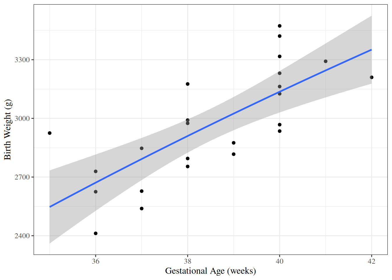
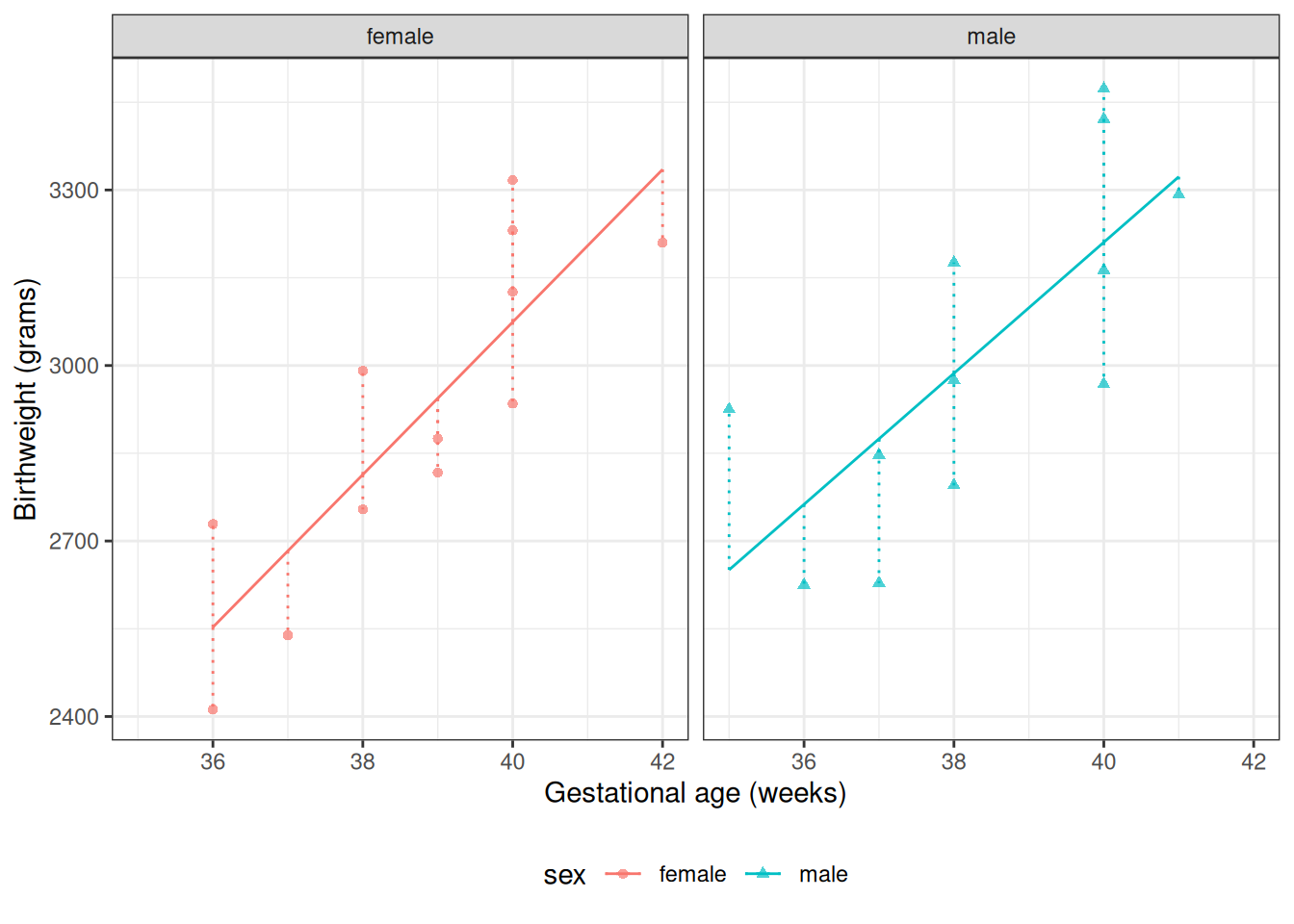
2.1 Motivating example: birthweights and gestational age

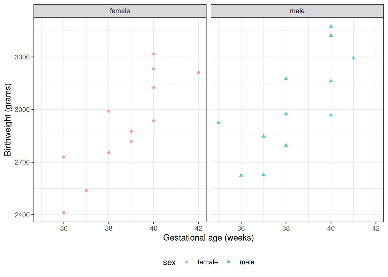
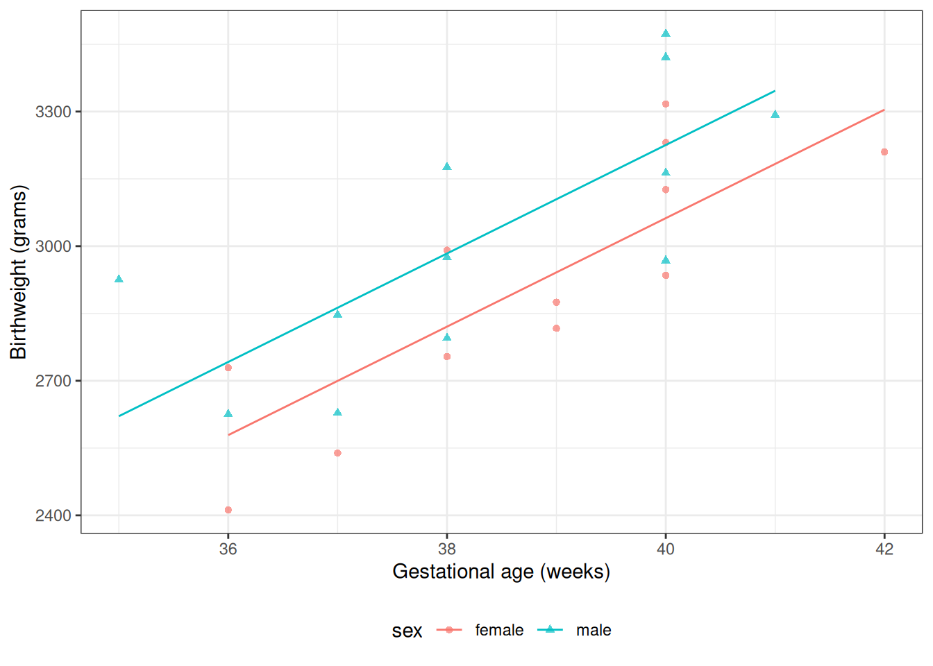
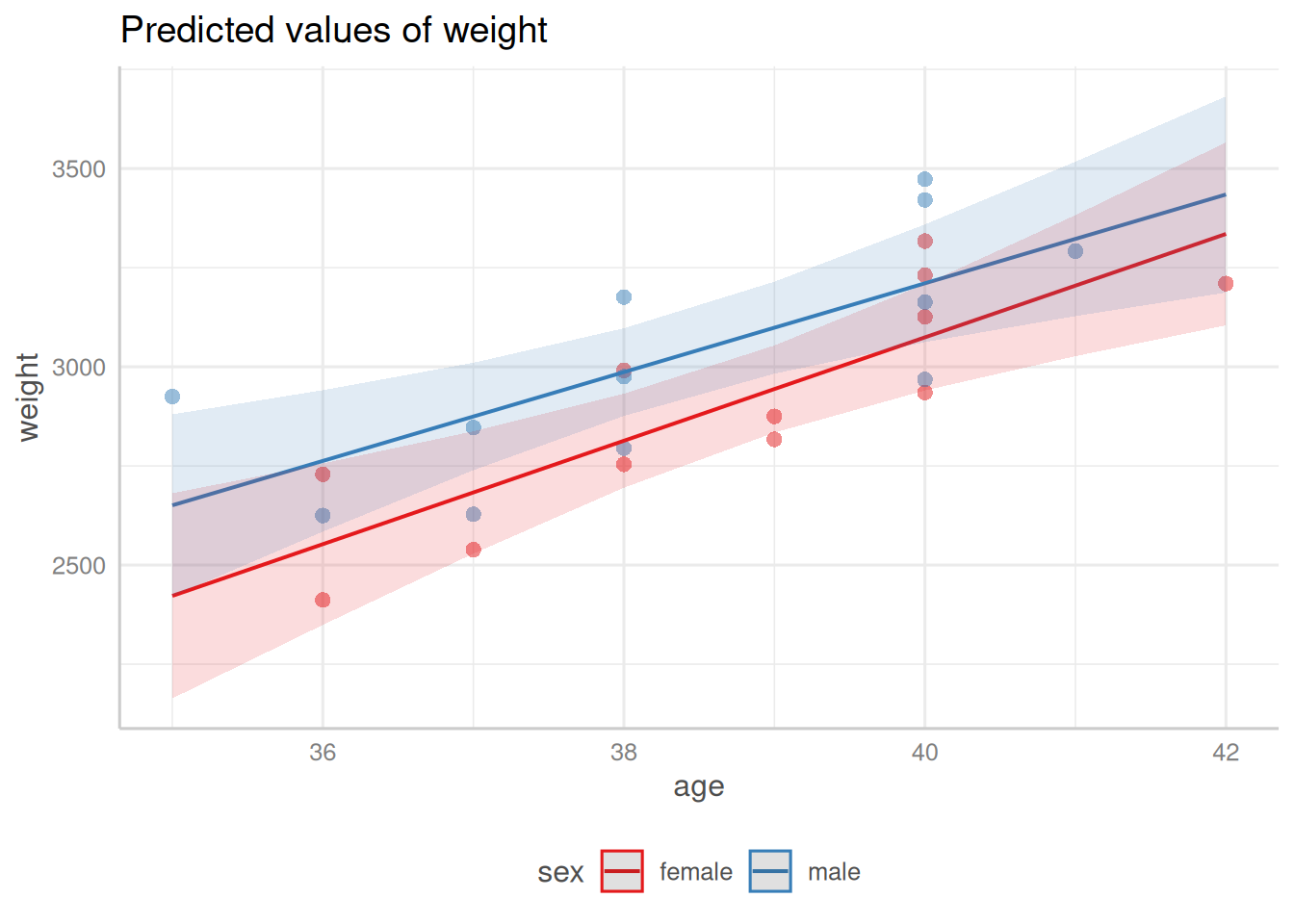
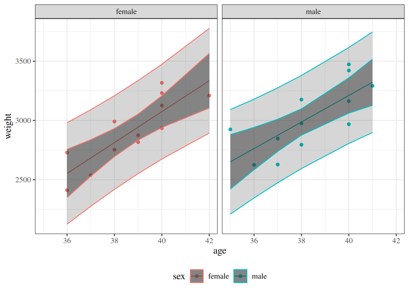
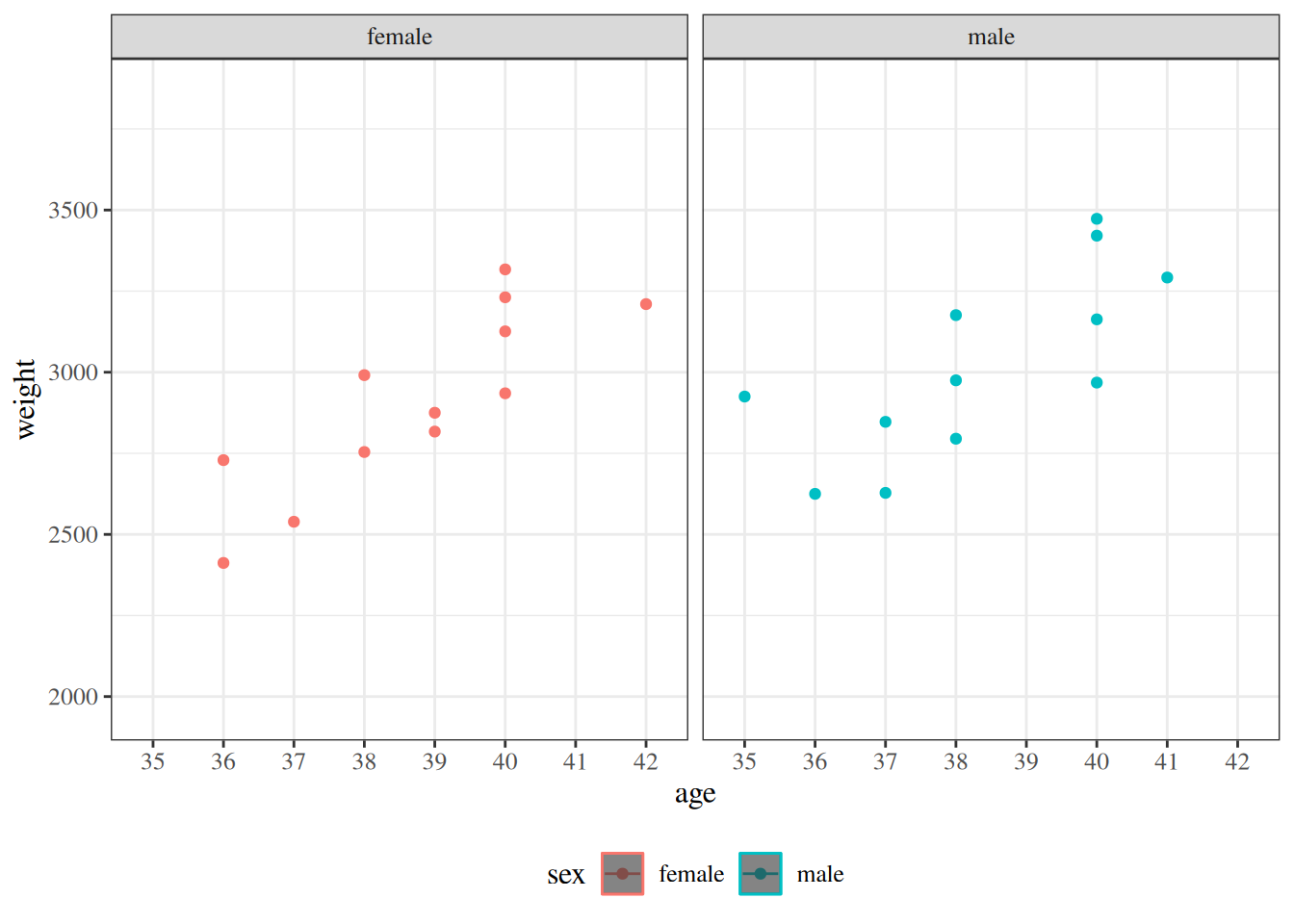
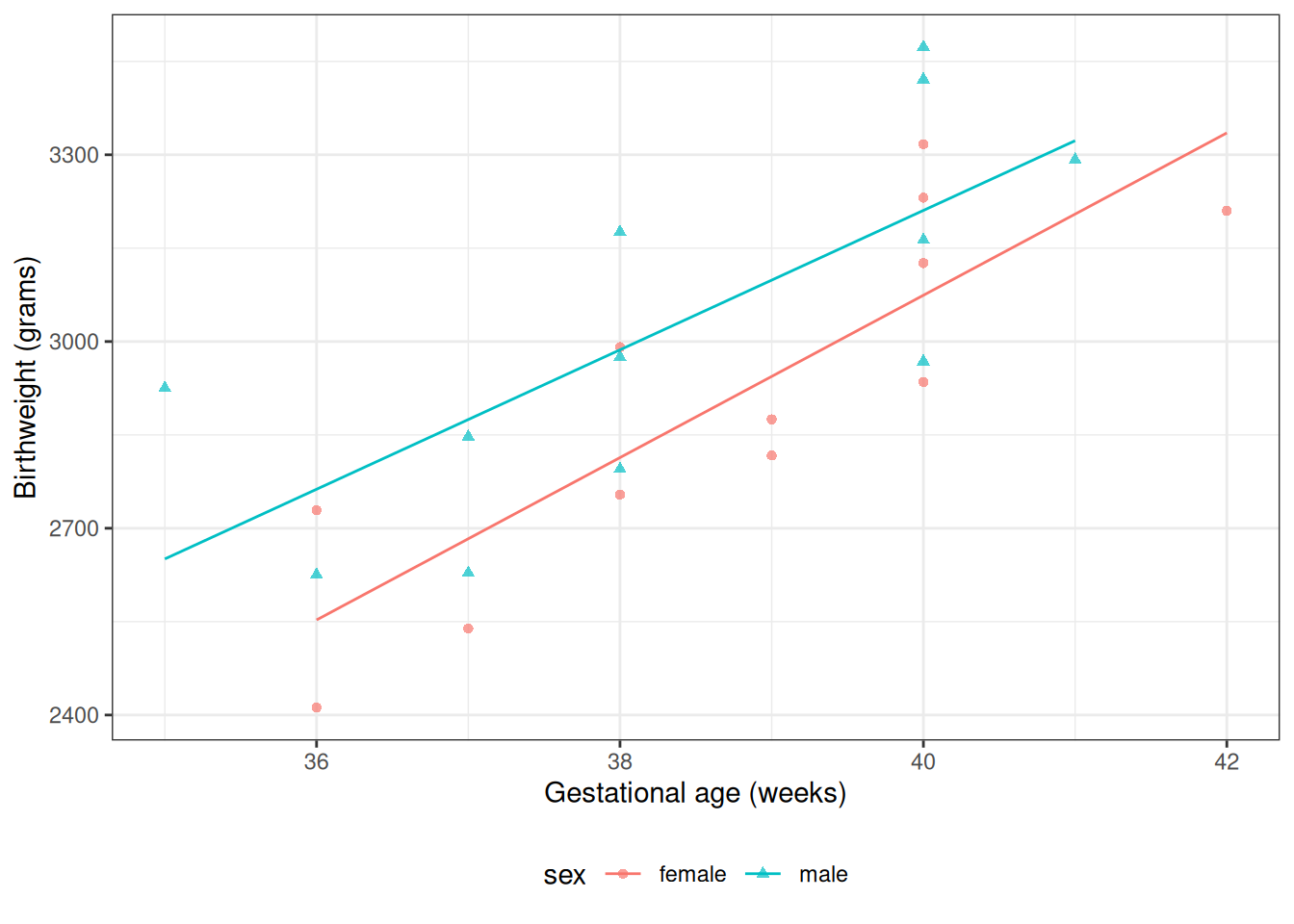
Suppose we want to learn about the distributions of birthweights (outcome \(Y\)) for (human) babies born at different gestational ages (covariate \(A\)) and with different chromosomal sexes (covariate \(S\)) (Dobson and Barnett (2018) Example 2.2.2).

2.2 Dobson birthweight data

• Data as table
• Reshape data for graphing
• Data as graph

library(dobson)
data("birthweight", package = "dobson")
birthweight

Table 1: birthweight data (Dobson and Barnett (2018) Example 2.2.2)

library(tidyverse)
bw <-
  birthweight |>
  pivot_longer(
    cols = everything(),
    names_to = c("sex", ".value"),
    names_sep = "s "
  ) |>
  rename(age = `gestational age`) |>
  mutate(
    id = row_number(),
    sex = sex |>
      case_match(
        "boy" ~ "male",
        "girl" ~ "female"
      ) |>
      factor(levels = c("female", "male")),
    male = sex == "male",
    female = sex == "female"
  )

bw

Table 2: birthweight data reshaped

plot1 <- bw |>
  ggplot(aes(
    x = age,
    y = weight,
    shape = sex,
    col = sex
  )) +
  theme_bw() +
  xlab("Gestational age (weeks)") +
  ylab("Birthweight (grams)") +
  theme(legend.position = "bottom") +
  # expand_limits(y = 0, x = 0) +
  geom_point(alpha = .7)
print(plot1 + facet_wrap(~sex))

Figure 1: birthweight data (Dobson and Barnett (2018) Example 2.2.2)

Data notation

Let’s define some notation to represent this data:

• \(Y\): birthweight (measured in grams)
• \(S\): chromosomal sex: “male” (XY) or “female” (XX)
• \(M\): indicator variable for \(S\) = “male”¹
• \(M = 0\) if \(S\) = “female”
• \(M = 1\) if \(S\) = “male”
• \(F\): indicator variable for \(S\) = “female”²
• \(F = 1\) if \(S\) = “female”
• \(F = 0\) if \(S\) = “male”
• \(A\): estimated gestational age at birth (measured in weeks).

Female is the reference level for the categorical variable \(S\) (chromosomal sex) and corresponding indicator variable \(M\) . The choice of a reference level is arbitrary and does not limit what we can do with the resulting model; it only makes it more computationally convenient to make inferences about comparisons involving that reference group.

\(M\) and \(F\) are called dummy variables; together, they are a numeric representation of the categorical variable \(S\). Dummy variables with values 0 and 1 are also called indicator variables. There are other ways to construct dummy variables, such as using the values -1 and 1 (see Dobson and Barnett (2018) §2.4 for details).

1. \(M\) is implicitly a deterministic function of \(S\)

2. \(F\) is implicitly a deterministic function of \(S\)

2.3 Parallel lines regression

(c.f. Dunn and Smyth (2018) §2.10.3)

We don’t have enough data to model the distribution of birth weight separately for each combination of gestational age and sex, so let’s instead consider a (relatively) simple model for how that distribution varies with gestational age and sex:

\[ \begin{aligned} Y|M,A &\ \sim_{\text{ciid}}\ N(\mu(M,A), \sigma^2)\\ \mu(m,a) &= \beta_0 + \beta_M m + \beta_A a \end{aligned} \tag{1}\]

Table 3 shows the parameter estimates from R. Figure 2 shows the estimated model, superimposed on the data.

bw_lm1 <- lm(
  formula = weight ~ sex + age,
  data = bw
)

library(parameters)
bw_lm1 |>
  parameters::parameters() |>
  parameters::print_md(
    include_reference = include_reference_lines,
    select = "{estimate}"
  )

Table 3: Regression parameter estimates for Model 1 of birthweight data

Parameter	Coefficient
(Intercept)	-1773.32
sex (male)	163.04
age	120.89

bw <-
  bw |>
  mutate(`E[Y|X=x]` = fitted(bw_lm1)) |>
  arrange(sex, age)

plot2 <-
  plot1 %+% bw +
  geom_line(aes(y = `E[Y|X=x]`))

print(plot2)

Figure 2: Graph of Model 1 for birthweight data

Model assumptions and predictions

To learn what this model is assuming, let’s plug in a few values.

Exercise 1 What’s the mean birthweight for a female born at 36 weeks?

Estimated coefficients for model 1

Parameter	Coefficient
(Intercept)	-1773.32
sex (male)	163.04
age	120.89

Solution.  

Estimated coefficients for model 1

Parameter	Coefficient
(Intercept)	-1773.32
sex (male)	163.04
age	120.89

pred_female <- coef(bw_lm1)["(Intercept)"] + coef(bw_lm1)["age"] * 36
## or using built-in prediction:
pred_female_alt <- predict(bw_lm1, newdata = tibble(sex = "female", age = 36))

\[ \begin{aligned} E[Y|M = 0, A = 36] &= \beta_0 + {\left(\beta_M \cdot 0\right)}+ {\left(\beta_A \cdot 36\right)} \\ &= -1773.321839 + {\left(163.039303 \cdot 0\right)} + {\left(120.894327 \cdot 36\right)} \\ &= 2578.873934 \end{aligned} \]

Exercise 2 What’s the mean birthweight for a male born at 36 weeks?

Estimated coefficients for model 1

Parameter	Coefficient
(Intercept)	-1773.32
sex (male)	163.04
age	120.89

Solution.  

Estimated coefficients for model 1

Parameter	Coefficient
(Intercept)	-1773.32
sex (male)	163.04
age	120.89

pred_male <-
  coef(bw_lm1)["(Intercept)"] +
  coef(bw_lm1)["sexmale"] +
  coef(bw_lm1)["age"] * 36

\[ \begin{aligned} E[Y|M = 1, A = 36] &= \beta_0 + \beta_M \cdot 1+ \beta_A \cdot 36 \\ &= 2741.913237 \end{aligned} \]

Exercise 3 What’s the difference in mean birthweights between males born at 36 weeks and females born at 36 weeks?

coef(bw_lm1)
#> (Intercept)     sexmale         age 
#>   -1773.322     163.039     120.894

Solution. \[ \begin{aligned} & E[Y|M = 1, A = 36] - E[Y|M = 0, A = 36]\\ &= 2741.913237 - 2578.873934\\ &= 163.039303 \end{aligned} \]

Shortcut:

\[ \begin{aligned} & E[Y|M = 1, A = 36] - E[Y|M = 0, A = 36]\\ &= (\beta_0 + \beta_M \cdot 1+ \beta_A \cdot 36) - (\beta_0 + \beta_M \cdot 0+ \beta_A \cdot 36) \\ &= \beta_M \\ &= 163.039303 \end{aligned} \]

Age cancels out in this difference. In other words, according to this model, the difference between females and males with the same gestational age is the same for every age.

This characteristic is an assumption of the model specified by Equation 1. It’s hardwired into the parametric model structure, even before we estimated values for those parameters.

Coefficient Interpretation

Recall Model 1:

\[ E[Y|M=m,A=a] = \mu(m,a) = \beta_0 + \beta_M m + \beta_A a \]

Slope (of the mean with respect to age) for males: \[ \begin{aligned} \frac{d}{da}\mu(1,a) &= \frac{d}{da}(\beta_0 + \beta_M 1 + \beta_A a)\\ &= \left(\frac{d}{da}\beta_0 + \frac{d}{da}\beta_M 1 + \frac{d}{da}\beta_A a\right)\\ &= (0 + 0 + \beta_A) \\ &= \beta_A \end{aligned} \]

Slope for females:

\[ \begin{aligned} \frac{d}{da}\mu(0,a) &= \frac{d}{da}(\beta_0 + \beta_M 0 + \beta_A a)\\ &= \left(\frac{d}{da}\beta_0 + \frac{d}{da}\beta_M 0 + \frac{d}{da}\beta_A a\right)\\ &= (0 + 0 + \beta_A) \\ &= \beta_A \end{aligned} \]

Exercise 4 What is the interpretation of \(\beta_A\) in Model 1?

Solution. \[ \begin{aligned} \frac{d}{da}\mu(m,a) &= \frac{d}{da}(\beta_0 + \beta_M m + {\color{red}\beta_A} a)\\ &= \left(\frac{d}{da}\beta_0 + \frac{d}{da}\beta_M m + \frac{d}{da}{\color{red}\beta_A} a\right)\\ &= (0 + 0 + {\color{red}\beta_A}) \\ &= {\color{red}\beta_A} \end{aligned} \]

Conclusion:

\[\beta_A = \frac{d}{da}\mu(m,a)\]

\(\beta_A\) is the slope of mean birthweight with respect to gestational age, adjusting for sex.

Or we can plug in the definition of slope:

\[\beta_A = E[Y|M = m, A = a+1] - E[Y|M = m, A = a]\]

Exchangeability and consistency have not been assessed; so we are not discussing potential outcomes (causality), only observed outcomes.

Exercise 5 What is the interpretation of \(\beta_M\) in Model 1?

Solution.

More precisely written: \[ \text{E}{\left[Y|M=m,A=a\right]} = \mu(m,a) = \bigg\{ \begin{matrix} \beta_0 + \beta_M m +\beta_A a, & \text{for } m\in {\left\{0,1\right\}} \\ \text{undefined}, & \text{for } m \notin {\left\{0,1\right\}} \end{matrix} \] The model is undefined for \(m \notin {\left\{0,1\right\}}\), so the derivative with respect to \(m\) doesn’t exist.

\[ \begin{aligned} E[Y|M = 1,A = a] &= \beta_0 + {\color{red}\beta_M} 1 + \beta_A a \\ & = \beta_0 + {\color{red}\beta_M} + \beta_A a \\ E[Y|M = 0,A = a] &= \beta_0 + {\color{red}\beta_M} 0 + \beta_A a \\ & = \beta_0 + \beta_A a \end{aligned} \] So: \[ \begin{aligned} E[Y|M = 1,A = a] - E[Y|M = 0,A = a] &= (\beta_0 + {\color{red}\beta_M} + \beta_A a) - (\beta_0 + \beta_A a) \\ &= {\color{red}\beta_M} \end{aligned} \] Therefore: \[ \begin{aligned} \beta_M &= E[Y|M = 1,A = a] - E[Y|M = 0,A = a]\\ & =\mu(1,a) - \mu(0,a)\\ \end{aligned} \]

In words: \(\beta_M\) is the difference in mean birthweight between males and females adjusting for age.

Exercise 6 \(\beta_0 = ?\)

Solution. \[ \begin{aligned} \text{E}{\left[Y|M = 0,A = 0\right]} &= \mu(0,0)\\ &= {\color{red}\beta_0} + \beta_M 0 + \beta_A 0\\ &= {\color{red}\beta_0}\\ {\color{red}\beta_0} &= \text{E}{\left[Y|M = 0,A = 0\right]} = \mu(0,0) \end{aligned} \]

\(\beta_0\) is the mean birthweight for a female with gestational age 0 weeks.

Motivating example: hers data

Note

This section is based on Vittinghoff et al. (2012), Chapter 4.

The “heart and estrogen/progestin study” (HERS) was a clinical trial of hormone therapy for prevention of recurrent heart attacks and death among 2,763 post-menopausal women with existing coronary heart disease (CHD) (Hulley et al. 1998).

library(haven)
hers <- haven::read_dta(
  paste0(
    "https://regression.ucsf.edu/sites/g/files",
    "/tkssra6706/f/wysiwyg/home/data/hersdata.dta"
  )
)

• Data as table
• Data as graph

hers |> head()

Table 4: hers data

library(ggplot2)
hers_scatter <-
  hers |>
  ggplot(aes(
    x = BMI,
    y = LDL,
    shape = HT,
    col = HT
  )) +
  theme_bw() +
  xlab("BMI (kg/m²)") +
  ylab("LDL cholesterol (mg/dL)") +
  theme(legend.position = "bottom") +
  geom_point(alpha = .3)
print(hers_scatter + facet_wrap(~HT))

Figure 3: hers data (Vittinghoff et al. (2012))

Data notation

Let’s define some notation to represent this data:

• \(Y\): LDL cholesterol (mg/dL)
• \(T\): hormone therapy treatment assignment (“placebo” or “hormone therapy”)
• \(H\): indicator variable for \(T\) = “hormone therapy”
  • \(H = 0\) if \(T\) = “placebo”
  • \(H = 1\) if \(T\) = “hormone therapy”
• \(B\): BMI (kg/m²)
• \(U\): statin use (“no” or “yes”)
• \(V\): indicator variable for \(U\) = “yes”
  • \(V = 0\) if \(U\) = “no”
  • \(V = 1\) if \(U\) = “yes”

“Placebo” is the reference level for the categorical variable \(T\), and “no” is the reference level for statin use \(U\). The choice of reference level is arbitrary; it only affects the interpretation of the intercept and corresponding indicator coefficients.

Parallel lines regression for hers data

We model the distribution of LDL cholesterol as a linear function of BMI, with a separate intercept for each treatment group:

\[ \begin{aligned} Y|H,B &\ \sim_{\text{ciid}}\ N(\mu(H,B), \sigma^2)\\ \mu(h,b) &= \beta_0 + \beta_H h + \beta_B b \end{aligned} \tag{2}\]

library(dplyr)
hers_lm1 <- lm(
  formula = LDL ~ HT + BMI,
  data = hers,
  na.action = na.exclude
)

library(parameters)
hers_lm1 |>
  parameters::parameters() |>
  parameters::print_md(
    include_reference = include_reference_lines,
    select = "{estimate}"
  )

Table 5: Regression parameter estimates for Model 2

Parameter	Coefficient
(Intercept)	133.09
HT (hormone therapy)	0.21
BMI	0.41

hers <-
  hers |>
  dplyr::mutate(`E[LDL|X=x]` = fitted(hers_lm1)) |>
  dplyr::arrange(HT, BMI)

hers_scatter2 <-
  hers_scatter +
  geom_line(data = hers, aes(y = `E[LDL|X=x]`))

print(hers_scatter2)

Figure 4: Graph of Model 2 for hers data

2.4 Interactions

What if we don’t like that parallel lines assumption?

Then we need to allow an “interaction” between age \(A\) and sex \(S\):

\[E[Y|S=s,A=a] = \beta_0 + \beta_A a+ \beta_M m + \beta_{AM} (a \cdot m) \tag{3}\]

Now, the slope of mean birthweight \(E[Y|A,S]\) with respect to gestational age \(A\) depends on the value of sex \(S\).

bw_lm2 <- lm(weight ~ sex + age + sex:age, data = bw)
bw_lm2 |>
  parameters() |>
  parameters::print_md(
    include_reference = include_reference_lines,
    select = "{estimate}"
  )

Table 6: Birthweight model with interaction term

Parameter	Coefficient
(Intercept)	-2141.67
sex (male)	872.99
age	130.40
sex (male) × age	-18.42

bw <-
  bw |>
  mutate(
    predlm2 = predict(bw_lm2)
  ) |>
  arrange(sex, age)

plot1_interact <-
  plot1 %+% bw +
  geom_line(aes(y = predlm2))

print(plot1_interact)

Figure 5: Birthweight model with interaction term

Now we can see that the lines aren’t parallel.

Here’s another way we could rewrite this model (by collecting terms involving \(S\)):

\[ E[Y|M,A] = \beta_0 + \beta_M M+ (\beta_A + \beta_{AM} M) A \]

If you want to understand a coefficient in a model with interactions, collect terms for the corresponding variable, and you will see which other covariates interact with the variable whose coefficient you are interested in. In this case, the association between \(A\) (age) varies between males and females (that is, by sex \(S\)). ¹ So the slope of \(Y\) with respect to \(A\) depends on the value of \(M\). According to this model, there is no such thing as “the slope of birthweight with respect to age”. There are two slopes, one for each sex. We can only talk about “the slope of birthweight with respect to age among males” and “the slope of birthweight with respect to age among females”. Then: each non-interaction slope coefficient is the difference in means per unit difference in its corresponding variable, when all interacting variables are set to 0.

1. some call this kind of variation “interaction” or “effect modification”, but “act”, “effect”, “modify”, and “by” all suggest causality, which we are not prepared to assess here; let’s try to avoid using causal terms, unless we are constructing a causal model.

To learn what this model is assuming, let’s plug in a few values.

Exercise 7 According to this model, what’s the mean birthweight for a female born at 36 weeks?

Parameter	Coefficient
(Intercept)	-2141.67
sex (male)	872.99
age	130.40
sex (male) × age	-18.42

Solution.  

Parameter	Coefficient
(Intercept)	-2141.67
sex (male)	872.99
age	130.40
sex (male) × age	-18.42

pred_female <- coef(bw_lm2)["(Intercept)"] + coef(bw_lm2)["age"] * 36

\[ E[Y|M = 0, A = 36] = \beta_0 + \beta_M \cdot 0+ \beta_A \cdot 36 + \beta_{AM} \cdot (0 * 36) = 2552.733333 \]

Exercise 8 What’s the mean birthweight for a male born at 36 weeks?

Parameter	Coefficient
(Intercept)	-2141.67
sex (male)	872.99
age	130.40
sex (male) × age	-18.42

Solution.  

Parameter	Coefficient
(Intercept)	-2141.67
sex (male)	872.99
age	130.40
sex (male) × age	-18.42

pred_male <-
  coef(bw_lm2)["(Intercept)"] +
  coef(bw_lm2)["sexmale"] +
  coef(bw_lm2)["age"] * 36 +
  coef(bw_lm2)["sexmale:age"] * 36

\[ \begin{aligned} E[Y|M = 1, A = 36] &= \beta_0 + \beta_M \cdot 1+ \beta_A \cdot 36 + \beta_{AM} \cdot 1 \cdot 36\\ &= 2762.706897 \end{aligned} \]

Exercise 9 What’s the difference in mean birthweights between males born at 36 weeks and females born at 36 weeks?

Solution. \[ \begin{aligned} & E[Y|M = 1, A = 36] - E[Y|M = 0, A = 36]\\ &= (\beta_0 + \beta_M \cdot 1+ \beta_A \cdot 36 + \beta_{AM} \cdot 1 \cdot 36)\\ &\ \ \ \ \ -(\beta_0 + \beta_M \cdot 0+ \beta_A \cdot 36 + \beta_{AM} \cdot 0 \cdot 36) \\ &= \beta_M + \beta_{AM}\cdot 36\\ &= 209.973563 \end{aligned} \]

Note that age now does show up in the difference: in other words, according to this model, the difference in mean birthweights between females and males with the same gestational age can vary by gestational age.

That’s how the lines in the graph ended up non-parallel.

Coefficient Interpretation

Exercise 10 What is the interpretation of \(\beta_{M}\) in Model 3?

Solution.  

Mean birthweight among males with gestational age 0 weeks: \[ \begin{aligned} \mu(1,0) &= \text{E}{\left[Y|M = 1,A = 0\right]}\\ &= \beta_0 + {\color{red}\beta_M} \cdot 1 + \beta_A \cdot 0 + \beta_{AM}\cdot 1 \cdot 0\\ &= \beta_0 + {\color{red}\beta_M} \end{aligned} \] Mean birthweight among females with gestational age 0 weeks: \[ \begin{aligned} \mu(0,0) &= \text{E}{\left[Y|M = 0,A = 0\right]}\\ &= \beta_0 + {\color{red}\beta_M} \cdot 0 + \beta_A \cdot 0 + \beta_{AM}\cdot 0 \cdot 0\\ &= \beta_0 \end{aligned} \]

\[ \begin{aligned} \beta_{M} &= \mu(1,0) - \mu(0,0) \\ &= \text{E}{\left[Y|M = 1,A = 0\right]} - \text{E}{\left[Y|M = 0,A = 0\right]} \end{aligned} \] \(\beta_M\) is the difference in mean birthweight between males with gestational age 0 weeks and females with gestational age 0 weeks.

Exercise 11 What is the interpretation of \(\beta_{AM}\) in Model 3?

Solution.  

Slope among males: \[ \begin{aligned} \frac{\partial}{\partial a}\mu(1,a) &= \frac{\partial}{\partial a}\left(\beta_0 + \beta_M\cdot1 + \beta_A\cdot a + {\color{red}\beta_{AM}}\cdot 1 \cdot a\right)\\ &= \frac{\partial}{\partial a}\left(\beta_0 + \beta_M + \beta_A\cdot a + {\color{red}\beta_{AM}} \cdot a\right)\\ &= \beta_A + {\color{red}\beta_{AM}} \end{aligned} \] or \[ \begin{aligned} E[Y|1,a+1] - E[Y|1,a] = &\beta_0 + \beta_M 1 + \beta_A(a+1) + {\color{red}\beta_{AM}}1(a+1)\\ &- (\beta_0 + \beta_M 1 + \beta_A(a) + {\color{red}\beta_{AM}}1(a))\\ = &\beta_A + {\color{red}\beta_{AM}} \end{aligned} \]

Slope among females: \[ \begin{aligned} \frac{\partial}{\partial a}\mu(0,a) &= \frac{\partial}{\partial a}\left(\beta_0 + \beta_M\cdot0 + \beta_A\cdot a + {\color{red}\beta_{AM}}\cdot 0 \cdot a\right)\\ &= \frac{\partial}{\partial a}\left(\beta_0 + \beta_A\cdot a\right)\\ &= \beta_A \\ \end{aligned} \] or \[ \begin{aligned} E[Y|0,a+1] - E[Y|0,a] = &\beta_0 + \beta_M0 + \beta_A(a+1) + {\color{red}\beta_{AM}}0(a+1) \\ &- (\beta_0 + \beta_M 0 + \beta_A(a) + {\color{red}\beta_{AM}}0(a))\\ = &\beta_0 + \beta_A(a+1) - (\beta_0 + \beta_A(a))\\ = &\beta_A \end{aligned} \]

Difference in slopes: \[ \begin{aligned} \frac{\partial}{\partial a}\mu(1,a) - \frac{\partial}{\partial a}\mu(0,a) &= \beta_A + {\color{red}\beta_{AM}} - \beta_A\\ &= {\color{red}\beta_{AM}} \end{aligned} \] or \[ \begin{aligned} (E[Y|1,a+1] - E[Y|1,a]) - (E[Y|0,a+1] - E[Y|0,a]) &= \beta_A + {\color{red}\beta_{AM}} - \beta_A\\ &= {\color{red}\beta_{AM}} \end{aligned} \]

Therefore \[ \begin{aligned} \beta_{AM} = &\frac{\partial}{\partial a}\mu(1,a) - \frac{\partial}{\partial a}\mu(0,a)\\ = &(E[Y|M = 1,A = a+1] - E[Y|M = 1,A = a])\\ &- (E[Y|M = 0,A = a+1] - E[Y|M = 0,A = a]) \end{aligned} \]

\(\beta_{AM}\) is the difference in slope of mean birthweight with respect to gestational age between males and females.

Compare coefficient interpretations

Table 7: Coefficient interpretations, by model structure

\(\mu(m,a)\)	\(\beta_0 + \beta_M m + \beta_A a\)	\(\beta_0 + \beta_M m + \beta_A a + {\color{red}\beta_{AM} ma}\)
\(\beta_0\)	\(\mu(0,0)\)	\(\mu(0,0)\)
\(\beta_A\)	\(\frac{\partial}{\partial a}\mu({\color{blue}m},a)\)	\(\frac{\partial}{\partial a}\mu({\color{red}0},a)\)
\(\beta_M\)	\(\mu(1, {\color{blue}a}) - \mu(0, {\color{blue}a})\)	\(\mu(1, {\color{red}0}) - \mu(0,{\color{red}0})\)
\(\beta_{AM}\)		\(\frac{\partial}{\partial a}\mu(1,a) - \frac{\partial}{\partial a}\mu(0,a)\)

In the model with an interaction term multiplying \(A\times M\), the interpretation of \(\beta_A\) involves the reference level of \(M\), and interpretation of \(\beta_M\) involves the reference level of \(A\) (Table 7).

Interactions in hers data

What if the slope of LDL with respect to BMI differs between statin users and non-users? Then we need an “interaction” between BMI \(B\) and statin use \(V\):

\[ \begin{aligned} Y|H,V,B &\ \sim_{\text{ciid}}\ N(\mu(H,V,B), \sigma^2)\\ \mu(h,v,b) &= \beta_0 + \beta_H h + \beta_V v + \beta_B b + \beta_{VB}(v \cdot b) \end{aligned} \tag{4}\]

Now the slope of mean LDL with respect to BMI \(B\) depends on statin use \(V\):

\[ \begin{aligned} \frac{\partial}{\partial b}\mu(H=h, V={\color{red}0}, B=b) &= \beta_B\\ \frac{\partial}{\partial b}\mu(H=h, V={\color{red}1}, B=b) &= \beta_B + \beta_{VB} \end{aligned} \]

hers_lm2 <- lm(
  LDL ~ HT + BMI + statins + BMI:statins,
  data = hers,
  na.action = na.exclude
)

hers_lm2 |>
  parameters() |>
  parameters::print_md(
    include_reference = include_reference_lines,
    select = "{estimate}"
  )

Table 8: HERS interaction model

Parameter	Coefficient
(Intercept)	132.86
HT (hormone therapy)	-0.10
BMI	0.64
statins (yes)	3.86
BMI × statins (yes)	-0.72

hers_scatter_statin <-
  hers |>
  ggplot(aes(
    x = BMI,
    y = LDL,
    shape = statins,
    col = statins
  )) +
  theme_bw() +
  xlab("BMI (kg/m²)") +
  ylab("LDL cholesterol (mg/dL)") +
  theme(legend.position = "bottom") +
  geom_point(alpha = .3)

hers <-
  hers |>
  dplyr::mutate(
    predlm2_hers = predict(hers_lm2)
  ) |>
  dplyr::arrange(statins, BMI)

hers_scatter_statin3 <-
  hers_scatter_statin +
  geom_line(data = hers, aes(y = predlm2_hers))

print(hers_scatter_statin3)

Figure 6: HERS interaction model fit (by statin use)

Graph of Model 4 for hers data

2.5 Stratified regression

We could re-write the interaction model as a stratified model, with a slope and intercept for each sex:

\[ \text{E}{\left[Y|A=a, S=s\right]} = \beta_M m + \beta_{AM} (a \cdot m) + \beta_F f + \beta_{AF} (a \cdot f) \tag{5}\]

Compare this stratified model (Equation 5) with our interaction model, Equation 3:

\[ \text{E}{\left[Y|A=a, S=s\right]} = \beta_0 + \beta_A a + \beta_M m + \beta_{AM} (a \cdot m) \]

In the stratified model, the intercept term \(\beta_0\) has been relabeled as \(\beta_F\).

bw_lm2 <- lm(weight ~ sex + age + sex:age, data = bw)
bw_lm2 |>
  parameters() |>
  print_md(
    include_reference = include_reference_lines,
    select = "{estimate}"
  )

Table 9: Birthweight model with interaction term

Parameter	Coefficient
(Intercept)	-2141.67
sex (male)	872.99
age	130.40
sex (male) × age	-18.42

bw_lm_strat <-
  bw |>
  lm(
    formula = weight ~ sex + sex:age - 1,
    data = _
  )

bw_lm_strat |>
  parameters() |>
  print_md(
    select = "{estimate}"
  )

Table 10: Birthweight model - stratified betas

Parameter	Coefficient
sex (female)	-2141.67
sex (male)	-1268.67
sex (female) × age	130.40
sex (male) × age	111.98

2.6 Curved-line regression

If we transform some of our covariates (\(X\)s) and plot the resulting model on the original covariate scale, we end up with curved regression lines:

bw_lm3 <- lm(weight ~ sex:log(age) - 1, data = bw)

ggbw <-
  bw |>
  ggplot(
    aes(x = age, y = weight)
  ) +
  geom_point() +
  xlab("Gestational Age (weeks)") +
  ylab("Birth Weight (g)")

ggbw2 <- ggbw +
  stat_smooth(
    method = "lm",
    formula = y ~ log(x),
    geom = "smooth"
  ) +
  xlab("Gestational Age (weeks)") +
  ylab("Birth Weight (g)")


ggbw2 |> print()

Figure 7: birthweight model with age entering on log scale

Below is an example with a slightly more obvious curve.

library(palmerpenguins)

ggpenguins <-
  palmerpenguins::penguins |>
  dplyr::filter(species == "Adelie") |>
  ggplot(
    aes(x = bill_length_mm, y = body_mass_g)
  ) +
  geom_point() +
  xlab("Bill length (mm)") +
  ylab("Body mass (g)")

ggpenguins2 <- ggpenguins +
  stat_smooth(
    method = "lm",
    formula = y ~ log(x),
    geom = "smooth"
  ) +
  xlab("Bill length (mm)") +
  ylab("Body mass (g)")


ggpenguins2 |> print()

Figure 8: palmerpenguins model with bill_length entering on log scale

2.7 Rescaling

Centering covariates (subtracting a constant from them) can make coefficient interpretations more meaningful, particularly for the intercept and main effect terms in models with interactions.

Rescale age

For example, the intercept \(\beta_0\) in our interaction model represents the mean birthweight for females at age = 0 weeks, which is not a biologically plausible scenario. If we center age at 36 weeks instead, \(\beta_0\) will represent the mean birthweight for females at 36 weeks, which is more interpretable.

Exercise 12 Let \(A^* = A - 32\) weeks.

Consider a new version of Model 3, with \(A^*\) in place of \(A\):

\[ \text{E}{\left[Y|M=m, A^*=a^*\right]} = \gamma_0 + \gamma_M m + \gamma_{A^*} a^* + \gamma_{A^*M} (m \cdot a^*) \tag{6}\]

Let the coefficients of this model be \(\gamma\)s instead of \(\beta\)s.

What are the interpretations of the \(\gamma\)s? How do they relate to the \(\beta\)s in Model 3? Which have the same interpretation? Which are different, and how do they differ? What is the pattern?

Solution. Interpretation of \(\gamma_0\):

From Model 6, \(\gamma_0\) is the mean birthweight among females (\(M = 0\)) with \(A^* = 0\) (i.e., \(A = 32\) weeks):

\[ \gamma_0 = \text{E}{\left[Y|M=0, A^*=0\right]} = \text{E}{\left[Y|M=0, A=32\right]} \]

Substituting into Model 3:

\[ \begin{aligned} \gamma_0 &= \beta_0 + \beta_M \cdot 0 + \beta_A \cdot 32 + \beta_{AM} \cdot 0 \cdot 32\\ &= \beta_0 + 32\beta_A \end{aligned} \]

This differs from \(\beta_0 = \text{E}{\left[Y|M=0, A=0\right]}\), which is the mean birthweight among females at \(A = 0\) weeks.

Interpretation of \(\gamma_M\):

From Model 6, \(\gamma_M\) is the sex difference in mean birthweight at \(A^* = 0\) (i.e., \(A = 32\) weeks):

\[ \begin{aligned} \gamma_M &= \text{E}{\left[Y|M=1, A^*=0\right]} - \text{E}{\left[Y|M=0, A^*=0\right]}\\ &= \text{E}{\left[Y|M=1, A=32\right]} - \text{E}{\left[Y|M=0, A=32\right]} \end{aligned} \]

Substituting into Model 3:

\[ \begin{aligned} \gamma_M &= (\beta_0 + \beta_M + \beta_A \cdot 32 + \beta_{AM} \cdot 32) - (\beta_0 + \beta_A \cdot 32)\\ &= \beta_M + 32\beta_{AM} \end{aligned} \]

This differs from \(\beta_M\), which is the sex difference at \(A = 0\) weeks.

Interpretation of \(\gamma_{A^*}\):

From Model 6, \(\gamma_{A^*}\) is the slope of mean birthweight with respect to \(A^*\) among females (\(M = 0\)):

\[ \begin{aligned} \gamma_{A^*} &= \frac{d}{da^*}\text{E}{\left[Y|M=0, A^*=a^*\right]}\\ &= \frac{d}{da^*}\text{E}{\left[Y|M=0, A=a^*+32\right]}\\ &= \frac{d}{da}\text{E}{\left[Y|M=0, A=a\right]} \end{aligned} \]

Substituting into Model 3:

\[ \begin{aligned} \gamma_{A^*} &= \frac{d}{da}\left(\beta_0 + \beta_A \cdot a\right)\\ &= \beta_A \end{aligned} \]

Since shifting \(A\) by a constant does not change the slope, \(\gamma_{A^*} = \beta_A\): these two coefficients have the same value and interpretation.

Interpretation of \(\gamma_{A^*M}\):

From Model 6, \(\gamma_{A^*M}\) is the difference in slope with respect to \(A^*\) between males and females:

\[ \begin{aligned} \gamma_{A^*M} &= \frac{d}{da^*}\text{E}{\left[Y|M=1, A^*=a^*\right]} - \frac{d}{da^*}\text{E}{\left[Y|M=0, A^*=a^*\right]}\\ &= \frac{d}{da}\text{E}{\left[Y|M=1, A=a\right]} - \frac{d}{da}\text{E}{\left[Y|M=0, A=a\right]} \end{aligned} \]

Substituting into Model 3:

\[ \begin{aligned} \gamma_{A^*M} &= (\beta_A + \beta_{AM}) - \beta_A\\ &= \beta_{AM} \end{aligned} \]

Since shifting \(A\) by a constant does not change slopes, \(\gamma_{A^*M} = \beta_{AM}\): these two coefficients have the same value and interpretation.

The pattern:

Slope coefficients (\(\gamma_{A^*}\) and \(\gamma_{A^*M}\)) are unchanged by rescaling: they have the same values and interpretations as the corresponding \(\beta\)s.

Coefficients change only for variables that have interactions with the rescaled variable \(A\). This includes the intercept (which can be viewed as the main effect of a variable that interacts with \(A\) via \(\beta_A\)), and the main effect of \(M\) (which interacts with \(A\) via \(\beta_{AM}\)). Shifting \(A\) by 32 weeks changes the reference point from \(A = 0\) to \(A = 32\), so these coefficients now represent quantities evaluated at \(A = 32\) weeks rather than at \(A = 0\) weeks.

Exercise 13 Using R, fit the rescaled interaction model with \(A^* = A - 36\) weeks in place of \(A\) in Model 3. Compare the coefficient estimates with those from the original model. Which coefficients change, and which remain the same?

Solution.

bw <-
  bw |>
  mutate(
    `age - mean` = age - mean(age),
    `age - 36wks` = age - 36
  )

lm1_c <- lm(weight ~ sex + `age - 36wks`, data = bw)

lm2_c <- lm(weight ~ sex + `age - 36wks` + sex:`age - 36wks`, data = bw)

parameters(lm2_c, ci_method = "wald") |> print_md()

Parameter	Coefficient	SE	95% CI	t(20)	p
(Intercept)	2552.73	97.59	(2349.16, 2756.30)	26.16	< .001
sex (male)	209.97	129.75	(-60.68, 480.63)	1.62	0.121
age - 36wks	130.40	30.00	(67.82, 192.98)	4.35	< .001
sex (male) × age - 36wks	-18.42	41.76	(-105.52, 68.68)	-0.44	0.664

Compare with what we got without rescaling:

parameters(bw_lm2, ci_method = "wald") |> print_md()

Parameter	Coefficient	SE	95% CI	t(20)	p
(Intercept)	-2141.67	1163.60	(-4568.90, 285.56)	-1.84	0.081
sex (male)	872.99	1611.33	(-2488.18, 4234.17)	0.54	0.594
age	130.40	30.00	(67.82, 192.98)	4.35	< .001
sex (male) × age	-18.42	41.76	(-105.52, 68.68)	-0.44	0.664

Notice that the slope coefficients (age - 36wks and sexmale:age - 36wks) remain the same, but the intercept and sexmale coefficient have changed to reflect means at age = 36 weeks rather than age = 0 weeks.

2.8 Categorical covariates with more than two levels

Example: birthweight

In the birthweight example, the variable sex had only two observed values:

unique(bw$sex)
#> [1] female male  
#> Levels: female male

If there are more than two observed values, we can’t just use a single variable with 0s and 1s.

Example: iris

For example, Table 11 shows the (in)famous iris data (Anderson (1935)), and Table 12 provides summary statistics. The data include three species: “setosa”, “versicolor”, and “virginica”.

head(iris)

Table 11: The iris data

library(table1)
table1(
  x = ~ . | Species,
  data = iris,
  overall = FALSE
)

Table 12: Summary statistics for the iris data

	setosa (N=50)	versicolor (N=50)	virginica (N=50)
Sepal.Length
Mean (SD)	5.01 (0.352)	5.94 (0.516)	6.59 (0.636)
Median [Min, Max]	5.00 [4.30, 5.80]	5.90 [4.90, 7.00]	6.50 [4.90, 7.90]
Sepal.Width
Mean (SD)	3.43 (0.379)	2.77 (0.314)	2.97 (0.322)
Median [Min, Max]	3.40 [2.30, 4.40]	2.80 [2.00, 3.40]	3.00 [2.20, 3.80]
Petal.Length
Mean (SD)	1.46 (0.174)	4.26 (0.470)	5.55 (0.552)
Median [Min, Max]	1.50 [1.00, 1.90]	4.35 [3.00, 5.10]	5.55 [4.50, 6.90]
Petal.Width
Mean (SD)	0.246 (0.105)	1.33 (0.198)	2.03 (0.275)
Median [Min, Max]	0.200 [0.100, 0.600]	1.30 [1.00, 1.80]	2.00 [1.40, 2.50]

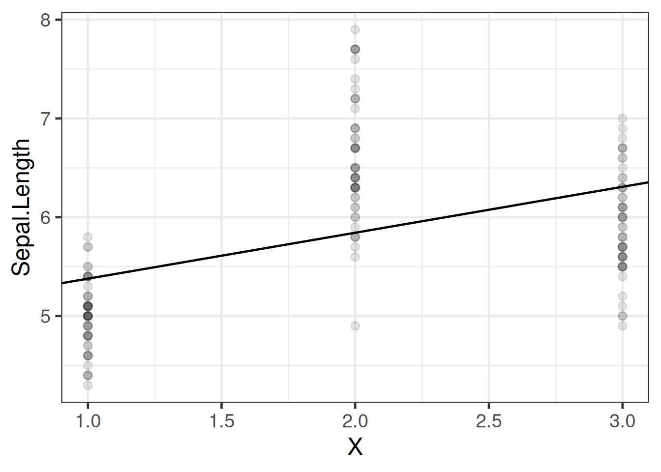
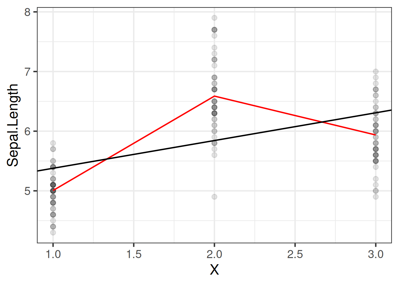
If we want to model Sepal.Length by species, we could create a variable \(X\) that represents “setosa” as \(X=1\), “virginica” as \(X=2\), and “versicolor” as \(X=3\).

data(iris) # this step is not always necessary, but ensures you're starting
# from the original version of a dataset stored in a loaded package

iris <-
  iris |>
  tibble() |>
  mutate(
    X = case_when(
      Species == "setosa" ~ 1,
      Species == "virginica" ~ 2,
      Species == "versicolor" ~ 3
    )
  )

iris |>
  distinct(Species, X)

Table 13: iris data with numeric coding of species

Then we could fit a model like:

iris_lm1 <- lm(Sepal.Length ~ X, data = iris)
iris_lm1 |>
  parameters() |>
  print_md()

Table 14: Model of iris data with numeric coding of Species

Parameter	Coefficient	SE	95% CI	t(148)	p
(Intercept)	4.91	0.16	(4.60, 5.23)	30.83	< .001
X	0.46	0.07	(0.32, 0.61)	6.30	< .001

Let’s see how that model looks:

iris_plot1 <- iris |>
  ggplot(
    aes(
      x = X,
      y = Sepal.Length
    )
  ) +
  geom_point(alpha = .1) +
  geom_abline(
    intercept = coef(iris_lm1)[1],
    slope = coef(iris_lm1)[2]
  ) +
  theme_bw(base_size = 18)
print(iris_plot1)

Figure 9: Model of iris data with numeric coding of Species

We have forced the model to use a straight line for the three estimated means. Maybe not a good idea?

Let’s see what R does with categorical variables by default:

iris_lm2 <- lm(Sepal.Length ~ Species, data = iris)
iris_lm2 |>
  parameters() |>
  print_md()

Table 15: Model of iris data with Species as a categorical variable

Parameter	Coefficient	SE	95% CI	t(147)	p
(Intercept)	5.01	0.07	(4.86, 5.15)	68.76	< .001
Species (versicolor)	0.93	0.10	(0.73, 1.13)	9.03	< .001
Species (virginica)	1.58	0.10	(1.38, 1.79)	15.37	< .001

Re-parametrize with no intercept

If you don’t want the default and offset option, you can use “-1” like we’ve seen previously:

iris_lm2_no_int <- lm(Sepal.Length ~ Species - 1, data = iris)
iris_lm2_no_int |>
  parameters() |>
  print_md()

Table 16

Parameter	Coefficient	SE	95% CI	t(147)	p
Species (setosa)	5.01	0.07	(4.86, 5.15)	68.76	< .001
Species (versicolor)	5.94	0.07	(5.79, 6.08)	81.54	< .001
Species (virginica)	6.59	0.07	(6.44, 6.73)	90.49	< .001

Let’s see what these new models look like:

iris_plot2 <-
  iris |>
  mutate(
    predlm2 = predict(iris_lm2)
  ) |>
  arrange(X) |>
  ggplot(aes(x = X, y = Sepal.Length)) +
  geom_point(alpha = .1) +
  geom_line(aes(y = predlm2), col = "red") +
  geom_abline(
    intercept = coef(iris_lm1)[1],
    slope = coef(iris_lm1)[2]
  ) +
  theme_bw(base_size = 18)

print(iris_plot2)

Figure 10

Let’s see how R did that:

formula(iris_lm2)
#> Sepal.Length ~ Species
model.matrix(iris_lm2) |>
  as_tibble() |>
  unique()

Table 17

This format is called a “corner point parametrization” (e.g., in Dobson and Barnett (2018)) or “treatment coding” (e.g., in Dunn and Smyth (2018)).

The default contrasts are controlled by options("contrasts"):

options("contrasts")
#> $contrasts
#>         unordered           ordered 
#> "contr.treatment"      "contr.poly"

See ?options for more details.

formula(iris_lm2_no_int)
#> Sepal.Length ~ Species - 1
model.matrix(iris_lm2_no_int) |>
  as_tibble() |>
  unique()

Table 18

This format is called a “group point parametrization” (e.g., in Dobson and Barnett (2018)).

There are more options; see Dobson and Barnett (2018) §6.4.1 and the codingMatrices package vignette (Venables (2023)).

2.9 Ordinal covariates

(c.f. Dobson and Barnett (2018) §2.4.4)

We can create ordinal variables in R using the ordered() function¹.

Example 1  

url <- paste0(
  "https://regression.ucsf.edu/sites/g/files/tkssra6706/",
  "f/wysiwyg/home/data/hersdata.dta"
)
library(haven)
hers <- read_dta(url)

hers |> head()

Table 19: HERS dataset

1. or equivalently, factor(ordered = TRUE)

For ordinal variables, we might want to use contrasts that respect the ordering of the categories. The default treatment contrasts don’t account for ordering.

Working with ordinal variables

When working with ordinal covariates in linear models:

1. Use ordered() or factor(ordered = TRUE) to create the variable
2. Consider using polynomial contrasts (contr.poly) which respect ordering
3. Alternatively, treat the ordinal variable as numeric if equal spacing is reasonable
4. Check ?codingMatrices::contr.diff for additional contrast options

See Dobson and Barnett (2018) §2.4.4 for more details on contrasts for ordinal variables.

3 Estimating Linear Models via Maximum Likelihood

In EPI 203 and our review of MLEs, we learned how to fit outcome-only models of the form \(p(X=x|\theta)\) to iid data \(\tilde{x}= (x_1,…,x_n)\) using maximum likelihood estimation.

Now, we apply the same procedure to linear regression models:

3.1 Likelihood

\[ \begin{aligned} \mathscr{L}_i &\stackrel{\text{def}}{=}p(Y_i=y_i|\tilde{X}_i = \tilde{x}_i) \\ &= (2\pi\sigma^2)^{-1/2} \text{exp}{\left\{-\frac{1}{2\sigma^2}\varepsilon_i^2\right\}} \\ \varepsilon_i &\stackrel{\text{def}}{=}y_i - \mu_i \\ \mu_i &\stackrel{\text{def}}{=}\mu(x_i) \\ &= x_i \cdot \beta \end{aligned} \]

\[ \begin{aligned} \mathscr{L}&\stackrel{\text{def}}{=}\mathscr{L}(\tilde{y}|\mathbf{x}, \tilde{\beta}, \sigma^2) \\ &\stackrel{\text{def}}{=}\text{p}(\tilde{Y}=\tilde{y}| \mathbf{X}= \mathbf{x}) \\ &= \prod_{i=1}^n \mathscr{L}_i \end{aligned} \tag{7}\]

3.2 Log-likelihood

\[ \begin{aligned} \ell_i &\stackrel{\text{def}}{=}\text{log}{\left\{\mathscr{L}_i\right\}} \\ &= \text{log}{\left\{(2\pi\sigma^2)^{-1/2} \text{exp}{\left\{-\frac{1}{2\sigma^2}\varepsilon_i^2\right\}}\right\}} \\ &= -\frac{1}{2}\text{log}{\left\{2\pi\sigma^2\right\}} -\frac{1}{2\sigma^2}\varepsilon_i^2 \end{aligned} \]

\[ \begin{aligned} \ell &\stackrel{\text{def}}{=}\ell(\tilde{y}|\mathbf{x},\beta, \sigma^2) \\ &\stackrel{\text{def}}{=}\text{log}{\left\{\mathscr{L}(\tilde{y}|\mathbf{x},\beta, \sigma^2)\right\}} \\ &= \text{log}{\left\{\prod_{i=1}^n\mathscr{L}_i\right\}} \\ &= \sum_{i=1}^n\text{log}{\left\{\mathscr{L}_i\right\}} \\ &= \sum_{i=1}^n\ell_i \\ &= \sum_{i=1}^n{\left(-\frac{1}{2}\text{log}{\left\{2\pi\sigma^2\right\}} -\frac{1}{2\sigma^2}\varepsilon_i^2\right)} \\ &= -\frac{n}{2}\text{log}{\left\{2\pi\sigma^2\right\}} - \frac{1}{2\sigma^2}\sum_{i=1}^n \varepsilon_i^2 \\ &= -\frac{n}{2}\text{log}{\left\{2\pi\sigma^2\right\}} - \frac{1}{2\sigma^2}{\left(\tilde{\varepsilon}\cdot \tilde{\varepsilon}\right)} \\ &= -\frac{n}{2}\text{log}{\left\{2\pi\sigma^2\right\}} - \frac{1}{2\sigma^2}{\left((\tilde{y}- \tilde{\mu}) \cdot (\tilde{y}- \tilde{\mu})\right)} \\ &= -\frac{n}{2}\text{log}{\left\{2\pi\sigma^2\right\}} - \frac{1}{2\sigma^2}{\left((\tilde{y}- \mathbf{X}\tilde{\beta}) \cdot (\tilde{y}- \mathbf{X}\tilde{\beta})\right)} \\ &= -\frac{n}{2}\text{log}{\left\{2\pi\sigma^2\right\}} - \frac{1}{2\sigma^2}\sum_{i=1}^n {\left(y_i - {\left(\tilde{x}_i\cdot \tilde{\beta}\right)}\right)}^2 \end{aligned} \tag{8}\]

3.3 Score function

\[ \begin{aligned} \mu_i' &\stackrel{\text{def}}{=}\frac{\partial}{\partial \tilde{\beta}} \mu_i \\ &= \frac{\partial}{\partial \tilde{\beta}} {\left(\tilde{x}_i \cdot \tilde{\beta}\right)} \\ &= {\left( \frac{\partial}{\partial \tilde{\beta}} \tilde{\beta}\right)} \tilde{x}_i \\ &= \mathbb{I}\tilde{x}_i \\ &= \tilde{x}_i \end{aligned} \]

\[ \begin{aligned} \varepsilon'_i &\stackrel{\text{def}}{=}\frac{\partial}{\partial \tilde{\beta}}\varepsilon_i \\ &= \frac{\partial}{\partial \tilde{\beta}} (y_i - \mu_i) \\ &= \frac{\partial}{\partial \tilde{\beta}}y_i - \frac{\partial}{\partial \tilde{\beta}} \mu_i \\ &= 0 - \tilde{x}_i \\ &= - \tilde{x}_i \end{aligned} \]

\[ \begin{aligned} \ell'_i &\stackrel{\text{def}}{=}\frac{\partial}{\partial \tilde{\beta}}\ell_i \\ &= \frac{\partial}{\partial \tilde{\beta}} {\left(-\frac{1}{2}\text{log}{\left\{2\pi\sigma^2\right\}} -\frac{1}{2\sigma^2}\varepsilon_i^2\right)} \\ &= \frac{\partial}{\partial \tilde{\beta}}{\left(-\frac{1}{2}\text{log}{\left\{2\pi\sigma^2\right\}}\right)} - \frac{\partial}{\partial \tilde{\beta}}\frac{1}{2\sigma^2}\varepsilon_i^2 \\ &= 0 - \frac{1}{2\sigma^2}\frac{\partial}{\partial \tilde{\beta}}\varepsilon_i^2 \\ &= - \frac{1}{2\sigma^2}2 {\left(\varepsilon_i'\right)} \varepsilon_i \\ &= - \frac{1}{\sigma^2} {\left(- \tilde{x}_i \varepsilon_i\right)} \\ &= \frac{1}{\sigma^2} \tilde{x}_i \varepsilon_i \end{aligned} \]

\[ \begin{aligned} \ell'_{\tilde{\beta}} &\stackrel{\text{def}}{=}\frac{\partial}{\partial \tilde{\beta}}\ell_{\tilde{\beta}} \\ &= \frac{\partial}{\partial \tilde{\beta}} \sum_{i=1}^n\ell_i \\ &= \sum_{i=1}^n\frac{\partial}{\partial \tilde{\beta}} \ell_i \\ &= \sum_{i=1}^n\ell_i' \\ &= \sum_{i=1}^n\frac{1}{\sigma^2} \tilde{x}_i \varepsilon_i \\ &= \frac{1}{\sigma^2} \sum_{i=1}^n\tilde{x}_i \varepsilon_i \\ &= \frac{1}{\sigma^2} \mathbf{X}^{\top} \tilde{\varepsilon} \end{aligned} \]

3.4 Hessian

\[ \begin{aligned} \ell_i'' &\stackrel{\text{def}}{=}\frac{\partial}{\partial \tilde{\beta}^{\top}}\frac{\partial}{\partial \tilde{\beta}} \ell_i \\ &= \frac{\partial}{\partial \tilde{\beta}^{\top}} \ell_i' \\ &= \frac{\partial}{\partial \tilde{\beta}^{\top}} {\left(\frac{1}{\sigma^2} \tilde{x}_i \varepsilon_i\right)} \\ &= \frac{1}{\sigma^2} \tilde{x}_i \varepsilon_i'^{\top} \\ &= \frac{1}{\sigma^2} \tilde{x}_i (-\tilde{x}_i^{\top}) \\ &= -\frac{1}{\sigma^2} \tilde{x}_i \tilde{x}_i^{\top} \end{aligned} \]

\[ \begin{aligned} \ell'' &\stackrel{\text{def}}{=}\frac{\partial}{\partial \tilde{\beta}^{\top}}\frac{\partial}{\partial \tilde{\beta}} \ell \\ &= \frac{\partial}{\partial \tilde{\beta}^{\top}} \ell' \\ &= \frac{\partial}{\partial \tilde{\beta}^{\top}} \sum_{i=1}^n\ell_i' \\ &= \sum_{i=1}^n\frac{\partial}{\partial \tilde{\beta}^{\top}} \ell_i' \\ &= \sum_{i=1}^n\ell_i'' \\ &= \sum_{i=1}^n-\frac{1}{\sigma^2} \tilde{x}_i \tilde{x}_i^{\top} \\ &= -\frac{1}{\sigma^2} \sum_{i=1}^n\tilde{x}_i \tilde{x}_i^{\top} \\ &= -\frac{1}{\sigma^2} \mathbf{X}^{\top}\mathbf{X} \end{aligned} \] That is,

\[\ell''= -\frac{1}{\sigma^2} \sum_{i=1}^n\tilde{x}_i \tilde{x}_i^{\top} \tag{9}\]

3.5 Alternative approach using matrix derivatives

\[ \begin{aligned} \ell'_{\tilde{\beta}}(\tilde{y}|\mathbf{x}, \tilde{\beta}, \sigma^2) &\stackrel{\text{def}}{=}\frac{\partial}{\partial \tilde{\beta}}\ell_{\tilde{\beta}}(\tilde{y}|\mathbf{x}, \tilde{\beta}, \sigma^2) \\ &= - \frac{1}{2\sigma^2}\frac{\partial}{\partial \tilde{\beta}} {\left(\sum_{i=1}^n {\left(y_i - {\left(\tilde{x}_i\cdot \tilde{\beta}\right)}\right)}^2\right)} \end{aligned} \tag{10}\]

Let’s switch to matrix-vector notation:

\[ \sum_{i=1}^n (y_i - \tilde{x}_i^{\top} \tilde{\beta})^2 = (\tilde{y}- \mathbf{X}\tilde{\beta}) \cdot (\tilde{y}- \mathbf{X}\tilde{\beta}) \]

So

\[ \begin{aligned} (\tilde{y}- \mathbf{X}\tilde{\beta})'(\tilde{y}- \mathbf{X}\tilde{\beta}) &= (\tilde{y}' - \tilde{\beta}'X')(\tilde{y}- \mathbf{X}\tilde{\beta}) \\ &= \tilde{y}'\tilde{y}- \tilde{\beta}'X'\tilde{y}- \tilde{y}'\mathbf{X}\tilde{\beta}+\tilde{\beta}'\mathbf{X}'\mathbf{X}\beta \\ &= \tilde{y}'\tilde{y}- 2\tilde{y}'\mathbf{X}\beta +\beta'\mathbf{X}'\mathbf{X}\beta \end{aligned} \]

We will use some results from vector calculus:

\[ \begin{aligned} \frac{\partial}{\partial \tilde{\beta}}{\left(\sum_{i=1}^n (y_i - x_i' \beta)^2\right)} &= \frac{\partial}{\partial \tilde{\beta}}(\tilde{y}- X\beta)'(\tilde{y}- X\beta) \\ &= \frac{\partial}{\partial \tilde{\beta}} (y'y - 2y'X\beta +\beta'\mathbf{X}'\mathbf{X}\beta) \\ &= (- 2X'y +2\mathbf{X}'\mathbf{X}\beta) \\ &= - 2X'(y - X\beta) \\ &= - 2X'(y - \text{E}[y]) \\ &= - 2X' \varepsilon(y) \end{aligned} \tag{11}\]

So if \(\ell'(\beta,\sigma^2) = 0\), then

\[ \begin{aligned} 0 &= (- 2X'y +2\mathbf{X}'\mathbf{X}\beta)\\ 2X'y &= 2\mathbf{X}'\mathbf{X}\beta\\ X'y &= \mathbf{X}'\mathbf{X}\beta\\ (\mathbf{X}'\mathbf{X})^{-1}X'y &= \beta \end{aligned} \]

Hessian

The Hessian (second derivative matrix) is:

\[ \begin{aligned} \ell_{\beta, \beta'} ''(\beta, \sigma^2;\tilde{y}, \mathbf{X}) &= -\frac{1}{2\sigma^2}\mathbf{X}'\mathbf{X} \end{aligned} \]

\(\ell_{\beta, \beta'} ''(\beta, \sigma^2;\mathbf X,\tilde{y})\) is negative definite at \(\beta = (\mathbf{X}'\mathbf{X})^{-1}X'y\), so \(\hat \beta_{ML} = (\mathbf{X}'\mathbf{X})^{-1}X'y\) is the MLE for \(\beta\).

Similarly (not shown):

\[ \hat\sigma^2_{ML} = \frac{1}{n} (Y-X\hat\beta)'(Y-X\hat\beta) \]

3.6 Residual Standard Deviation

\(\hat \sigma\) represents an estimate of the Residual Standard Deviation parameter, \(\sigma\). We can extract \(\hat \sigma\) from the fitted model, using the sigma() function:

sigma(bw_lm2)
#> [1] 180.613

\(\sigma\) is NOT “Residual standard error”

In the summary.lm() output, this estimate is labeled as "Residual standard error":

summary(bw_lm2)
#> 
#> Call:
#> lm(formula = weight ~ sex + age + sex:age, data = bw)
#> 
#> Residuals:
#>    Min     1Q Median     3Q    Max 
#> -246.7 -138.1  -39.1  176.6  274.3 
#> 
#> Coefficients:
#>             Estimate Std. Error t value Pr(>|t|)    
#> (Intercept)  -2141.7     1163.6   -1.84  0.08057 .  
#> sexmale        873.0     1611.3    0.54  0.59395    
#> age            130.4       30.0    4.35  0.00031 ***
#> sexmale:age    -18.4       41.8   -0.44  0.66389    
#> ---
#> Signif. codes:  0 '***' 0.001 '**' 0.01 '*' 0.05 '.' 0.1 ' ' 1
#> 
#> Residual standard error: 181 on 20 degrees of freedom
#> Multiple R-squared:  0.643,  Adjusted R-squared:  0.59 
#> F-statistic:   12 on 3 and 20 DF,  p-value: 0.000101

However, this is a misnomer: see note in ?stats::sigma

4 Inference about Gaussian Linear Regression Models

4.1 Motivating example: birthweight data

Research question: is there really an interaction between sex and age?

\(H_0: \beta_{AM} = 0\)

\(H_A: \beta_{AM} \neq 0\)

\(P(|\hat\beta_{AM}| > |-18.417241| \mid H_0)\) = ?

4.2 Inference for individual predictor coefficients

Sampling distribution of \(\hat\beta\)

The Fisher information for \(\beta\) is:

\[ \begin{aligned} \mathcal I_{\beta} &= \text{E}{\left[-\ell_{\beta, \beta'}''(Y|X,\beta, \sigma^2)\right]}\\ &= \frac{1}{\sigma^2}\mathbf{X}'\mathbf{X} \end{aligned} \]

Therefore:

\[ \text{Var}{\left(\hat \beta\right)} \approx (\mathcal I_{\beta})^{-1} = \sigma^2 (\mathbf{X}'\mathbf{X})^{-1} \]

and

\[ \hat\beta \dot \sim N(\beta, \mathcal I_{\beta}^{-1}) \]

These are all results you have hopefully seen before.

In the Gaussian linear regression case, we also have exact results:

\[ \frac{\hat\beta_j}{\widehat{\text{se}}{\left(\hat\beta_j\right)}} \ \sim \ t_{n-p} \]

Estimated covariance matrix and standard errors

Example 2 (MLEs for birthweight data) In model 3 above, \(\hat{\mathcal{I}}(\beta)\) is:

bw_lm2 |> vcov()
#>             (Intercept)  sexmale        age sexmale:age
#> (Intercept)     1353968 -1353968 -34870.966   34870.966
#> sexmale        -1353968  2596387  34870.966  -67210.974
#> age              -34871    34871    899.896    -899.896
#> sexmale:age       34871   -67211   -899.896    1743.548

Table 20: Covariance matrix of \(\hat{\tilde{\beta}}\) for birthweight model 3 (with interaction term)

If we take the square roots of the diagonals, we get the standard errors listed in the model output:

bw_lm2 |>
  vcov() |>
  diag() |>
  sqrt()
#> (Intercept)     sexmale         age sexmale:age 
#>   1163.6015   1611.3309     29.9983     41.7558

bw_lm2 |>
  parameters() |>
  print_md()

Table 21: Estimated model for birthweight data with interaction term

Parameter	Coefficient	SE	95% CI	t(20)	p
(Intercept)	-2141.67	1163.60	(-4568.90, 285.56)	-1.84	0.081
sex (male)	872.99	1611.33	(-2488.18, 4234.17)	0.54	0.594
age	130.40	30.00	(67.82, 192.98)	4.35	< .001
sex (male) × age	-18.42	41.76	(-105.52, 68.68)	-0.44	0.664

So we can do confidence intervals, hypothesis tests, and p-values exactly as in the one-variable case we looked at previously.

Wald tests and confidence intervals

For Gaussian linear regression, the ordinary least squares (OLS) estimates \(\hat\beta_k\) are exactly Gaussian when the error terms \(\epsilon_i\) are Gaussian, for any sample size. See also the table of Gaussian vs. MLE-based tests.

Wald test statistic

To test \(H_0: \beta_k = \beta_{k,0}\) (typically \(\beta_{k,0} = 0\)):

\[t_k = \frac{\hat\beta_k - \beta_{k,0}}{\widehat{SE}(\hat\beta_k)}\]

Under \(H_0\), \(t_k \sim t_{n-p}\) exactly when errors are Gaussian.

Confidence intervals for regression coefficients

A 95% confidence interval for \(\beta_k\) is:

\[\hat\beta_k \pm t_{n-p}(0.975) \cdot \widehat{SE}(\hat\beta_k)\]

In R

In R, parameters() from the parameters package automatically computes Wald tests and confidence intervals for linear regression model coefficients:

bw_lm2 |>
  parameters() |>
  print_md(
    include_reference = TRUE
  )

Table 22: Wald tests and 95% CIs for birthweight linear regression

Parameter	Coefficient	SE	95% CI	t(20)	p
(Intercept)	-2141.67	1163.60	(-4568.90, 285.56)	-1.84	0.081
sex (female)	0.00
sex (male)	872.99	1611.33	(-2488.18, 4234.17)	0.54	0.594
age	130.40	30.00	(67.82, 192.98)	4.35	< .001
sex (male) × age	-18.42	41.76	(-105.52, 68.68)	-0.44	0.664

To understand what’s happening, let’s replicate these results by hand for the interaction term.

P-values

bw_lm2 |>
  parameters(keep = "sexmale:age") |>
  print_md(
    include_reference = TRUE
  )

Parameter	Coefficient	SE	95% CI	t(20)	p
sex (male) × age	-18.42	41.76	(-105.52, 68.68)	-0.44	0.664

beta_hat <- coef(summary(bw_lm2))["sexmale:age", "Estimate"]
se_hat <- coef(summary(bw_lm2))["sexmale:age", "Std. Error"]
dfresid <- bw_lm2$df.residual
t_stat <- abs(beta_hat) / se_hat
pval_t <-
  pt(-t_stat, df = dfresid, lower.tail = TRUE) +
  pt(t_stat, df = dfresid, lower.tail = FALSE)

\[ \begin{aligned} &P{\left( | \hat \beta_{AM} | > | -18.417241| \middle| H_0 \right)} \\ &= \Pr {\left( \left| \frac{\hat\beta_{AM}}{\hat{SE}(\hat\beta_{AM})} \right| > \left| \frac{-18.417241}{41.755817} \right| \middle| H_0 \right)}\\ &= \Pr {\left( \left| T_{20} \right| > 0.44107 | H_0 \right)}\\ &= 0.663893 \end{aligned} \]

This matches the result in the table above.

Confidence intervals

q_t_upper <- qt(
  p = 0.975,
  df = dfresid,
  lower.tail = TRUE
)

q_t_lower <- qt(
  p = 0.025,
  df = dfresid,
  lower.tail = TRUE
)

confint_radius_t <-
  se_hat * q_t_upper

confint_t <- beta_hat + c(-1, 1) * confint_radius_t

print(confint_t)
#> [1] -105.5184   68.6839

This also matches.

Gaussian approximations

For large samples, the t-distribution is well-approximated by the standard Gaussian:

pval_z <- pnorm(abs(t_stat), lower.tail = FALSE) * 2

print(pval_z)
#> [1] 0.659162

confint_radius_z <- se_hat * qnorm(0.975, lower.tail = TRUE)
confint_z <-
  beta_hat + c(-1, 1) * confint_radius_z
print(confint_z)
#> [1] -100.2571   63.4227

4.3 Inference for predicted means

Exercise 14 Given a maximum likelihood estimate \(\hat{\tilde{\beta}}\) and a corresponding estimated covariance matrix \(\hat \Sigma\stackrel{\text{def}}{=}\widehat{\text{Cov}}(\hat{\tilde{\beta}})\), calculate a 95% confidence interval for the predicted mean \(\mu(\tilde{x}) = \text{E}{\left[Y|\tilde{X}=\tilde{x}\right]}\).

Solution 1.

By the Gauss-Markov theorem, the OLS estimate \(\hat{\tilde{\beta}}\) is the best linear unbiased estimator of \(\tilde{\beta}\). A 95% confidence interval for \(\mu(\tilde{x})\) can be constructed directly on the original scale:

\[\hat\mu(\tilde{x}) \pm t_{n-p}(0.975) \cdot \widehat{\text{SE}}{\left(\hat\mu(\tilde{x})\right)}\]

where \(\hat\mu(\tilde{x}) = \tilde{x}'\hat{\tilde{\beta}}\).

Unlike in logistic regression, no transformation is needed; the confidence interval is constructed directly on the mean scale.

\[\mu(\tilde{x}) \in {\left(\hat\mu(\tilde{x}) \pm t_{n-p}(0.975) \cdot \widehat{\text{SE}}{\left(\hat\mu(\tilde{x})\right)}\right)}\]

Exercise 15  

How can we estimate the standard error of \(\hat\mu(\tilde{x})\)?

\[{\color{blue}\widehat{\text{SE}}{\left(\hat\mu(\tilde{x})\right)}} = {\color{blue}?}\]

Solution 2. \[ {\color{green}\text{SE}{\left(\hat\mu(\tilde{x})\right)}} = \sqrt{{\color{red}\text{Var}{\left(\hat\mu(\tilde{x})\right)}}} \tag{12}\]

By the definition \(\hat\mu(\tilde{x}) = \tilde{x}'\hat{\tilde{\beta}}\) and the variance of a linear combination:

\[ \begin{aligned} {\color{red}\text{Var}{\left(\hat\mu(\tilde{x})\right)}} &= \text{Var}{\left(\tilde{x}'\hat{\tilde{\beta}}\right)} \\ &= \tilde{x}'\text{Cov}{\left(\hat{\tilde{\beta}}\right)}\tilde{x} \\ &= {\color{red}{\tilde{x}}^{\top}\Sigma\tilde{x}} \end{aligned} \tag{13}\]

where \(\Sigma \stackrel{\text{def}}{=}\text{Cov}(\hat{\tilde{\beta}})\).

---

Expanding Equation 13 out of matrix-vector notation, we have:

\[ \begin{aligned} {\color{red}{\tilde{x}}^{\top}\Sigma\tilde{x}} &= \sum_{i=1}^p\sum_{j=1}^px_i \Sigma_{ij} x_j \\ &= {\color{red}\sum_{i=1}^p\sum_{j=1}^px_i \text{Cov}(\hat{\tilde{\beta}}_i,\hat{\tilde{\beta}}_j) x_j} \end{aligned} \]

---

Combining Equation 13 and the Gauss-Markov theorem:

Theorem 1 (Estimated variance and standard error of predicted mean) \[ {\color{orange}\widehat{\text{Var}}{\left(\hat\mu(\tilde{x})\right)}} = {\color{orange}{\tilde{x}}^{\top}\hat{\Sigma}\tilde{x}} \tag{14}\]

\[ {\color{blue}\widehat{\text{SE}}{\left(\hat\mu(\tilde{x})\right)}} = {\color{blue}\sqrt{{\tilde{x}}^{\top}\hat{\Sigma}\tilde{x}}} \tag{15}\]

Note: on the RHS, we have plugged in \(\hat{\Sigma}\), our estimate of \(\Sigma\).

In R

In R, predict() with se.fit = TRUE computes the estimated mean \(\hat\mu(\tilde{x}) = \tilde{x}'\hat{\tilde{\beta}}\) and its estimated standard error for each covariate pattern:

library(dplyr)
new_data <- tibble(
  age = c(36, 38, 40),
  sex = "male"
)

pred_mean <-
  bw_lm2 |>
  predict(
    newdata = new_data,
    se.fit = TRUE
  )

new_data |>
  mutate(
    mu_hat = pred_mean$fit,
    se = pred_mean$se.fit,
    ci_lower = mu_hat - qt(0.975, df = bw_lm2$df.residual) * se,
    ci_upper = mu_hat + qt(0.975, df = bw_lm2$df.residual) * se
  ) |>
  knitr::kable(digits = 3)

Table 23: Predicted means and 95% CI for birthweight linear regression

age	sex	mu_hat	se	ci_lower	ci_upper
36	male	2762.71	85.508	2584.34	2941.07
38	male	2986.67	53.030	2876.05	3097.29
40	male	3210.64	71.147	3062.23	3359.05

Alternatively, predict() with interval = "confidence" gives the same result:

bw_lm2 |>
  predict(
    newdata = new_data,
    interval = "confidence"
  ) |>
  cbind(new_data) |>
  knitr::kable(digits = 3)

Table 24: Predicted means and 95% CI using interval = 'confidence'

fit	lwr	upr	age	sex
2762.71	2584.34	2941.07	36	male
2986.67	2876.05	3097.29	38	male
3210.64	3062.23	3359.05	40	male

4.4 Inference for differences in means

Exercise 16 Given a maximum likelihood estimate \(\hat{\tilde{\beta}}\) and a corresponding estimated covariance matrix \(\hat \Sigma\stackrel{\text{def}}{=}\widehat{\text{Cov}}(\hat{\tilde{\beta}})\), calculate a 95% confidence interval for the difference in means comparing covariate patterns \(\tilde{x}\) and \({\tilde{x}^*}\), \(\mu(\tilde{x}) - \mu({\tilde{x}^*})\).

Solution 3.

The difference in means is a linear function of \(\hat{\tilde{\beta}}\), so we can construct the confidence interval directly:

\[\widehat{\mu(\tilde{x}) - \mu({\tilde{x}^*})} \pm t_{n-p}(0.975) \cdot \widehat{\text{SE}}{\left(\widehat{\mu(\tilde{x}) - \mu({\tilde{x}^*})}\right)}\]

No transformation is needed (unlike for odds ratios in logistic regression).

\[\mu(\tilde{x}) - \mu({\tilde{x}^*}) \in {\left(\widehat{\mu(\tilde{x}) - \mu({\tilde{x}^*})} \pm t_{n-p}(0.975) \cdot \widehat{\text{SE}}{\left(\widehat{\mu(\tilde{x}) - \mu({\tilde{x}^*})}\right)}\right)}\]

Exercise 17 Express the difference in means \(\mu(\tilde{x}) - \mu({\tilde{x}^*})\) as a linear function of \(\tilde{\beta}\).

Solution 4. \[ \begin{aligned} \mu(\tilde{x}) - \mu({\tilde{x}^*}) &= {\tilde{x}}^{\top}\tilde{\beta}- {({\tilde{x}^*})}^{\top}\tilde{\beta} \\ &= (\tilde{x}- {\tilde{x}^*})'\tilde{\beta} \\ &= \Delta\tilde{x}'\tilde{\beta} \end{aligned} \tag{16}\]

where \(\Delta\tilde{x}\stackrel{\text{def}}{=}\tilde{x}- {\tilde{x}^*}\).

Exercise 18  

How can we estimate the standard error of \(\widehat{\mu(\tilde{x}) - \mu({\tilde{x}^*})}\)?

\[{\color{blue}\widehat{\text{SE}}{\left(\widehat{\mu(\tilde{x}) - \mu({\tilde{x}^*})}\right)}} = {\color{blue}?}\]

Solution 5. \[ {\color{green}\text{SE}{\left(\widehat{\mu(\tilde{x}) - \mu({\tilde{x}^*})}\right)}} = \sqrt{{\color{red}\text{Var}{\left(\widehat{\mu(\tilde{x}) - \mu({\tilde{x}^*})}\right)}}} \tag{17}\]

By Solution 4 and the variance of a linear combination:

\[ \begin{aligned} {\color{red}\text{Var}{\left(\widehat{\mu(\tilde{x}) - \mu({\tilde{x}^*})}\right)}} &= \text{Var}{\left((\Delta\tilde{x})'\hat{\tilde{\beta}}\right)} \\ &= {\left(\Delta\tilde{x}\right)}^{\top}\text{Cov}{\left(\hat{\tilde{\beta}}\right)}(\Delta\tilde{x}) \\ &= {\color{red}{\left(\Delta\tilde{x}\right)}^{\top}\Sigma(\Delta\tilde{x})} \end{aligned} \tag{18}\]

where \(\Sigma \stackrel{\text{def}}{=}\text{Cov}(\hat{\tilde{\beta}})\).

---

Expanding Equation 18 out of matrix-vector notation, we have:

\[ \begin{aligned} {\color{red}{\left(\Delta\tilde{x}\right)}^{\top}\Sigma(\Delta\tilde{x})} &= \sum_{i=1}^p\sum_{j=1}^p(\Delta\tilde{x})_i \Sigma_{ij} (\Delta\tilde{x})_j \\ &= \sum_{i=1}^p\sum_{j=1}^p(\Delta x_i) \Sigma_{ij} (\Delta x_j) \\ &= {\color{red}\sum_{i=1}^p\sum_{j=1}^p(x_i - x^*_i) \text{Cov}(\hat{\tilde{\beta}}_i,\hat{\tilde{\beta}}_j) (x_j - x^*_j)} \end{aligned} \]

---

Combining Equation 18 and the Gauss-Markov theorem:

Theorem 2 (Estimated variance and standard error of difference in means) \[ {\color{orange}\widehat{\text{Var}}{\left(\widehat{\mu(\tilde{x}) - \mu({\tilde{x}^*})}\right)}} = {\color{orange}{\Delta\tilde{x}}^{\top}\hat{\Sigma}(\Delta\tilde{x})} \tag{19}\]

\[ {\color{blue}\widehat{\text{SE}}{\left(\widehat{\mu(\tilde{x}) - \mu({\tilde{x}^*})}\right)}} = {\color{blue}\sqrt{{\Delta\tilde{x}}^{\top}\hat{\Sigma}(\Delta\tilde{x})}} \tag{20}\]

Note: on the RHS, we have plugged in \(\hat{\Sigma}\), our estimate of \(\Sigma\).

Compare this result with the formula for inference for predicted means: the only change is to replace \(\tilde{x}\) with \(\Delta\tilde{x}= \tilde{x}- {\tilde{x}^*}\).

In R

In R, we can compute the CI for the difference in means by computing the predicted means for both covariate patterns and applying the variance formula directly:

library(dplyr)
new_data_pair <- tibble(
  sex = factor(c("female", "male"), levels = levels(bw$sex)),
  age = c(40, 40)
)

pred_pair <-
  bw_lm2 |>
  predict(
    newdata = new_data_pair,
    se.fit = TRUE
  )

design_mat <- model.matrix(delete.response(terms(bw_lm2)), new_data_pair)
delta_x <- design_mat[2, ] - design_mat[1, ]

sigma_hat <- vcov(bw_lm2)

diff_mean_hat <- diff(pred_pair$fit)
se_diff <- sqrt(t(delta_x) %*% sigma_hat %*% delta_x)
t_crit <- qt(0.975, df = bw_lm2$df.residual)

tibble(
  diff_mean = diff_mean_hat,
  se = as.numeric(se_diff),
  ci_lower = diff_mean_hat - t_crit * se,
  ci_upper = diff_mean_hat + t_crit * se
) |>
  knitr::kable(digits = 3)

Table 25: 95% CI for difference in birthweight means (male vs. female)

diff_mean	se	ci_lower	ci_upper
136.305	95.846	-63.626	336.236

4.5 Likelihood ratio statistics

logLik(bw_lm2)
#> 'log Lik.' -156.579 (df=5)
logLik(bw_lm1)
#> 'log Lik.' -156.695 (df=4)

log_LR <- (logLik(bw_lm2) - logLik(bw_lm1)) |> as.numeric()
delta_df <- (bw_lm1$df.residual - df.residual(bw_lm2))


x_max <- 1

d_log_LR <- function(x, df = delta_df) dchisq(x, df = df)

chisq_plot <-
  ggplot() +
  geom_function(fun = d_log_LR) +
  stat_function(
    fun = d_log_LR,
    xlim = c(log_LR, x_max),
    geom = "area",
    fill = "gray"
  ) +
  geom_segment(
    aes(
      x = log_LR,
      xend = log_LR,
      y = 0,
      yend = d_log_LR(log_LR)
    ),
    col = "red"
  ) +
  xlim(0.0001, x_max) +
  ylim(0, 4) +
  ylab("p(X=x)") +
  xlab("log(likelihood ratio) statistic [x]") +
  theme_classic()
chisq_plot |> print()

Figure 11: Chi-square distribution

Now we can get the p-value:

pchisq(
  q = 2 * log_LR,
  df = delta_df,
  lower = FALSE
) |>
  print()
#> [1] 0.629806

In practice you don’t have to do this by hand; there are functions to do it for you:

# built in
library(lmtest)
lrtest(bw_lm2, bw_lm1)

5 Prediction

5.1 Prediction for linear models

Definition 1 (Predicted value) In a regression model \(\text{p}(y|\tilde{x})\), the predicted value of \(y\) given \(\tilde{x}\) is the estimated mean of \(Y\) given \(\tilde{X}=\tilde{x}\):

\[\hat y \stackrel{\text{def}}{=}\hat{\text{E}}{\left[Y|\tilde{X}=\tilde{x}\right]}\]

For linear models, the predicted value can be straightforwardly calculated by multiplying each predictor value \(x_j\) by its corresponding coefficient \(\beta_j\) and adding up the results:

\[ \begin{aligned} \hat y &= \hat{\text{E}}{\left[Y|\tilde{X}=\tilde{x}\right]} \\ &= \tilde{x}'\hat\beta \\ &= \hat\beta_0\cdot 1 + \hat\beta_1 x_1 + ... + \hat\beta_p x_p \end{aligned} \]

5.2 Example: prediction for the birthweight data

x <- c(1, 1, 40)
sum(x * coef(bw_lm1))
#> [1] 3225.49

R has built-in functions for prediction:

x <- tibble(age = 40, sex = "male")
bw_lm1 |> predict(newdata = x)
#>       1 
#> 3225.49

If you don’t provide newdata, R will use the covariate values from the original dataset:

predict(bw_lm1)
#>       1       2       3       4       5       6       7       8       9      10 
#> 3225.49 3062.45 2983.70 2578.87 3225.49 3062.45 2621.02 2820.66 2741.91 3304.24 
#>      11      12      13      14      15      16      17      18      19      20 
#> 2862.81 2941.56 3346.38 3062.45 3225.49 2699.77 2862.81 2578.87 2983.70 2820.66 
#>      21      22      23      24 
#> 3225.49 2941.56 2983.70 3062.45

These special predictions are called the fitted values of the dataset:

Definition 2 For a given dataset \((\tilde{Y}, \mathbf{X})\) and corresponding fitted model \(\text{p}_{\hat \beta}(\tilde{y}|\mathbf{x})\), the fitted value of \(y_i\) is the predicted value of \(y\) when \(\tilde{X}=\tilde{x}_i\) using the estimate parameters \(\hat \beta\).

R has an extra function to get these values:

fitted(bw_lm1)
#>       1       2       3       4       5       6       7       8       9      10 
#> 3225.49 3062.45 2983.70 2578.87 3225.49 3062.45 2621.02 2820.66 2741.91 3304.24 
#>      11      12      13      14      15      16      17      18      19      20 
#> 2862.81 2941.56 3346.38 3062.45 3225.49 2699.77 2862.81 2578.87 2983.70 2820.66 
#>      21      22      23      24 
#> 3225.49 2941.56 2983.70 3062.45

5.3 Confidence intervals

Use predict(se.fit = TRUE) to compute SEs for predicted values:

bw_lm1 |>
  predict(
    newdata = x,
    se.fit = TRUE
  )
#> $fit
#>       1 
#> 3225.49 
#> 
#> $se.fit
#> [1] 61.4599
#> 
#> $df
#> [1] 21
#> 
#> $residual.scale
#> [1] 177.116

The output of predict.lm(se.fit = TRUE) is a list(); you can extract the elements with $ or magrittr::use_series():

library(magrittr)
bw_lm1 |>
  predict(
    newdata = x,
    se.fit = TRUE
  ) |>
  use_series(se.fit)
#> [1] 61.4599

We can construct confidence intervals for \(\text{E}{\left[Y|X=x\right]}\) using the usual formula:

\[\mu(\tilde{x}) \in {\left({\color{red}\hat{\mu}(\tilde{x})} \pm {\color{blue}\zeta_\alpha}\right)}\]

\[ {\color{blue}\zeta_\alpha} = t_{n-p}{\left(1-\frac{\alpha}{2}\right)} * \widehat{\text{se}}{\left(\hat{\mu}(\tilde{x})\right)} \]

\[{\color{red}\hat{\mu}(\tilde{x})} = \tilde{x}\cdot \hat \beta\]

\[\text{se}{\left(\hat{\mu}(\tilde{x})\right)} = \sqrt{\text{Var}{\left(\hat{\mu}(\tilde{x})\right)}}\] \[ \begin{aligned} \text{Var}{\left(\hat{\mu}(\tilde{x})\right)} &= \text{Var}{\left(x'\hat{\beta}\right)} \\&= x' \text{Var}{\left(\hat{\beta}\right)} x \\&= x' \sigma^2(\mathbf{X}'\mathbf{X})^{-1} x \\&= \sigma^2 x' (\mathbf{X}'\mathbf{X})^{-1} x \\&= \sum_{i=1}^n\sum_{j=1}^nx_i x_j \text{Cov}{\left(\hat \beta_i, \hat \beta_j\right)} \end{aligned} \] \[\widehat{\text{Var}}{\left(\hat{\mu}(\tilde{x})\right)} = \hat \sigma^2 x' (\mathbf{X}'\mathbf{X})^{-1} x\]

bw_lm2 |> predict(
  newdata = x,
  interval = "confidence"
)
#>       fit     lwr     upr
#> 1 3210.64 3062.23 3359.05

library(sjPlot)
bw_lm2 |>
  plot_model(type = "pred", terms = c("age", "sex"), show.data = TRUE) +
  theme_sjplot() +
  theme(legend.position = "bottom")

Figure 12: Predicted values and confidence bands for the birthweight model with interaction term

5.4 Prediction intervals

We can also construct prediction intervals for the value of a new observation \(Y^*\), given a covariate pattern \({\tilde{x}^*}\).

A new observation \(Y^*\) at \({\tilde{x}^*}\) follows the same linear model as the training data:

\[Y^* = {({\tilde{x}^*})}^{\top}\tilde{\beta}+ \varepsilon^*\]

where \(\varepsilon^* \sim \text{N}{\left(0, \sigma^2\right)}\) is independent of the training data (and therefore independent of \(\hat \beta\)).

The predicted value of \(Y^*\) is:

\[\hat{Y}^* \stackrel{\text{def}}{=}\hat\mu({\tilde{x}^*}) = {({\tilde{x}^*})}^{\top}\hat \beta\]

We base the prediction interval on the prediction error \(Y^* - \hat{Y}^*\):

\[ \begin{aligned} Y^* - \hat{Y}^* &= {({\tilde{x}^*})}^{\top}\tilde{\beta}+ \varepsilon^* - {({\tilde{x}^*})}^{\top}\hat \beta \\ &= \varepsilon^* - {({\tilde{x}^*})}^{\top}(\hat \beta- \tilde{\beta}) \end{aligned} \]

The prediction error is unbiased:

\[ \begin{aligned} \text{E}{\left[Y^* - \hat{Y}^*\right]} &= \text{E}{\left[\varepsilon^*\right]} - {({\tilde{x}^*})}^{\top}\text{E}{\left[\hat \beta- \tilde{\beta}\right]} \\ &= 0 - {({\tilde{x}^*})}^{\top} \cdot 0 \\ &= 0 \end{aligned} \]

The variance of the prediction error is:

\[ \begin{aligned} \text{Var}{\left(Y^* - \hat{Y}^*\right)} &= \text{Var}{\left(\varepsilon^* - {({\tilde{x}^*})}^{\top}(\hat \beta- \tilde{\beta})\right)} \\ &= \text{Var}{\left(\varepsilon^*\right)} + \text{Var}{\left({({\tilde{x}^*})}^{\top}\hat \beta\right)} \quad \text{(since } \varepsilon^* \perp\!\!\!\perp\hat \beta\text{)} \\ &= \sigma^2 + {({\tilde{x}^*})}^{\top}\text{Var}{\left(\hat \beta\right)}{\tilde{x}^*} \\ &= \sigma^2 + {({\tilde{x}^*})}^{\top}{\left(\sigma^2(\mathbf{X}'\mathbf{X})^{-1}\right)}{\tilde{x}^*} \\ &= \sigma^2 + \sigma^2{({\tilde{x}^*})}^{\top}(\mathbf{X}'\mathbf{X})^{-1}{\tilde{x}^*} \\ &= \sigma^2{\left(1 + {({\tilde{x}^*})}^{\top}(\mathbf{X}'\mathbf{X})^{-1}{\tilde{x}^*}\right)} \end{aligned} \tag{21}\]

See Hogg et al. (2015) §7.6 (p. 340).

bw_lm2 |>
  predict(newdata = x, interval = "predict")
#>       fit     lwr     upr
#> 1 3210.64 2805.71 3615.57

If you don’t specify newdata, you get a warning:

bw_lm2 |>
  predict(interval = "predict") |>
  head()
#> Warning in predict.lm(bw_lm2, interval = "predict"): predictions on current data refer to _future_ responses
#>       fit     lwr     upr
#> 1 2552.73 2124.50 2980.97
#> 2 2552.73 2124.50 2980.97
#> 3 2683.13 2275.99 3090.27
#> 4 2813.53 2418.60 3208.47
#> 5 2813.53 2418.60 3208.47
#> 6 2943.93 2551.48 3336.38

The warning from the last command is: “predictions on current data refer to future responses” (since you already know what happened to the current data, and thus don’t need to predict it).

See ?predict.lm for more.

library(rlang) # defines the `.data` pronoun
plot_PIs_and_CIs <- function(data, model = NULL) {
  if (is.null(model)) {
    rlang::abort("`model` must be supplied to `plot_PIs_and_CIs()`.")
  }

  if (!is.data.frame(data) && is.data.frame(model)) {
    rlang::warn(
      paste0(
        "`plot_PIs_and_CIs()` received `model` as the first argument ",
        "and `data` as the second. ",
        "Please update the call to use `data` first and `model` second."
      )
    )
    tmp <- data
    data <- model
    model <- tmp
  }

  cis <- model |>
    predict(newdata = data, interval = "confidence") |>
    suppressWarnings() |>
    tibble::as_tibble()
  names(cis) <- paste("ci", names(cis), sep = "_")

  preds <- model |>
    predict(newdata = data, interval = "predict") |>
    suppressWarnings() |>
    tibble::as_tibble()
  names(preds) <- paste("pred", names(preds), sep = "_")
  dplyr::bind_cols(data, cis, preds) |>
    ggplot2::ggplot() +
    ggplot2::aes(
      x = .data$age,
      y = .data$weight,
      col = .data$sex
    ) +
    ggplot2::geom_point() +
    ggplot2::theme(legend.position = "bottom") +
    ggplot2::geom_line(ggplot2::aes(y = .data$ci_fit)) +
    ggplot2::geom_ribbon(
      ggplot2::aes(
        ymin = .data$pred_lwr,
        ymax = .data$pred_upr
      ),
      alpha = 0.2
    ) +
    ggplot2::geom_ribbon(
      ggplot2::aes(
        ymin = .data$ci_lwr,
        ymax = .data$ci_upr
      ),
      alpha = 0.5
    ) +
    ggplot2::facet_wrap(~sex)
}

plot_PIs_and_CIs(bw, bw_lm2)

Figure 13: Confidence and prediction intervals for birthweight model 3

6 Assessing model fit

6.1 Goodness of fit

AIC and BIC

This section is adapted from Vittinghoff et al. (2012, sec. 4.5) and Kleinbaum et al. (2014, sec. 15).

When we use likelihood ratio tests, we are comparing how well different models fit the data.

Likelihood ratio tests require nested models: one must be a special case of the other.

AIC and BIC can be used to compare both nested and non-nested models.

Formulas

Definition 3 (Akaike Information Criterion (AIC)) \[\text{AIC} = -2 \ell(\hat\theta) + 2 p\]

where \(\ell(\hat\theta)\) is the log-likelihood evaluated at the maximum-likelihood estimates \(\hat\theta\), \(p\) is the number of estimated parameters (including \(\hat\sigma^2\) for Gaussian models), and \(n\) is the number of observations.

Definition 4 (Bayesian Information Criterion (BIC)) \[\text{BIC} = -2 \ell(\hat\theta) + p \log(n)\]

where \(\ell(\hat\theta)\), \(p\), and \(n\) are defined as in Definition 3.

Conceptual basis

Each criterion has two components:

• Fit term (\(-2\ell(\hat\theta)\)): measures lack of fit — lower is better. A model with more parameters will always achieve a higher (or equal) log-likelihood on the observed data.

• Penalty term (\(2 p\) for AIC; \(p \log(n)\) for BIC): penalizes model complexity to guard against overfitting.

Together, they balance goodness of fit against parsimony.

The AIC was introduced by Akaike (1974) and is grounded in information theory (specifically, the Kullback-Leibler divergence). The BIC was introduced by Schwarz (1978) as an approximation to the Bayes factor for model comparison.

AIC vs. BIC

Criterion	Penalty per parameter	Tends to select
AIC	\(2\)	larger models
BIC	\(\log(n)\)	smaller models

The BIC penalty exceeds the AIC penalty whenever \(\log(n) > 2\), i.e., when \(n > e^2 \approx 7.4\). In practice, BIC almost always penalizes additional parameters more heavily than AIC and therefore tends to select simpler (more parsimonious) models (Vittinghoff et al. 2012; Kleinbaum et al. 2014).

AIC in R

-2 * logLik(bw_lm2) |> as.numeric() +
  2 * (length(coef(bw_lm2)) + 1) # sigma counts as a parameter here
#> [1] 323.159

AIC(bw_lm2)
#> [1] 323.159

BIC in R

-2 * logLik(bw_lm2) |> as.numeric() +
  (length(coef(bw_lm2)) + 1) * log(nobs(bw_lm2))
#> [1] 329.049

BIC(bw_lm2)
#> [1] 329.049

Interpretation

• Lower values are better. There are no hypothesis tests or p-values associated with these criteria.

• To compare models, calculate the criterion for each model and choose the model with the smallest value.

• Differences of less than 2 units are generally considered negligible; differences greater than 10 are considered strong evidence in favor of the lower-criterion model.

• BIC tends to favor simpler models than AIC, especially when the sample size is large.

(Residual) Deviance

Let \(q\) be the number of distinct covariate combinations in a data set.

bw_X_unique <-
  bw |>
  count(sex, age)

n_unique_bw <- nrow(bw_X_unique)

For example, in the birthweight data, there are \(q = 12\) unique patterns (Table 26).

bw_X_unique

Table 26: Unique covariate combinations in the birthweight data, with replicate counts

Definition 5 (Replicates) If a given covariate pattern has more than one observation in a dataset, those observations are called replicates.

Example 3 (Replicates in the birthweight data) In the birthweight dataset, there are 2 replicates of the combination “female, age 36” (Table 26).

Exercise 19 (Replicates in the birthweight data) Which covariate pattern(s) in the birthweight data has the most replicates?

Solution 6 (Replicates in the birthweight data). Two covariate patterns are tied for most replicates: males at age 40 weeks and females at age 40 weeks. 40 weeks is the usual length for human pregnancy (Polin et al. (2011)), so this result makes sense.

bw_X_unique |> dplyr::filter(n == max(n))

Saturated models

The most complicated model we could fit would have one parameter (a mean) for each covariate pattern, plus a variance parameter:

lm_max <-
  bw |>
  mutate(age = factor(age)) |>
  lm(
    formula = weight ~ sex:age - 1,
    data = _
  )

lm_max |>
  parameters() |>
  print_md()

Table 27: Saturated model for the birthweight data

Parameter	Coefficient	SE	95% CI	t(12)	p
sex (male) × age35	2925.00	187.92	(2515.55, 3334.45)	15.56	< .001
sex (female) × age36	2570.50	132.88	(2280.98, 2860.02)	19.34	< .001
sex (male) × age36	2625.00	187.92	(2215.55, 3034.45)	13.97	< .001
sex (female) × age37	2539.00	187.92	(2129.55, 2948.45)	13.51	< .001
sex (male) × age37	2737.50	132.88	(2447.98, 3027.02)	20.60	< .001
sex (female) × age38	2872.50	132.88	(2582.98, 3162.02)	21.62	< .001
sex (male) × age38	2982.00	108.50	(2745.60, 3218.40)	27.48	< .001
sex (female) × age39	2846.00	132.88	(2556.48, 3135.52)	21.42	< .001
sex (female) × age40	3152.25	93.96	(2947.52, 3356.98)	33.55	< .001
sex (male) × age40	3256.25	93.96	(3051.52, 3460.98)	34.66	< .001
sex (male) × age41	3292.00	187.92	(2882.55, 3701.45)	17.52	< .001
sex (female) × age42	3210.00	187.92	(2800.55, 3619.45)	17.08	< .001

We call this model the full, maximal, or saturated model for this dataset.

Figure 14: Model 3 and saturated model for birthweight data, with confidence and prediction intervals

plot_PIs_and_CIs(bw, bw_lm2)

(a) Model 3 (linear with age:sex interaction)

plot_PIs_and_CIs(bw |> mutate(age = factor(age)), lm_max)

(b) Saturated model

We can calculate the log-likelihood of this model as usual:

logLik(lm_max)
#> 'log Lik.' -151.402 (df=13)

We can compare this model to our other models using chi-square tests, as usual:

lrtest(lm_max, bw_lm2)

The likelihood ratio statistic for this test is \[\lambda = 2 * (\ell_{\text{full}} - \ell) = 10.355374\] where:

• \(\ell_{\text{full}}\) is the log-likelihood of the full model: -151.401601
• \(\ell\) is the log-likelihood of our comparison model (two slopes, two intercepts): -156.579288

This statistic is called the deviance or residual deviance for our two-slopes and two-intercepts model; it tells us how much the likelihood of that model deviates from the likelihood of the maximal model.

The corresponding p-value tells us whether there we have enough evidence to detect that our two-slopes, two-intercepts model is a worse fit for the data than the maximal model; in other words, it tells us if there’s evidence that we missed any important patterns. (Remember, a nonsignificant p-value could mean that we didn’t miss anything and a more complicated model is unnecessary, or it could mean we just don’t have enough data to tell the difference between these models.)

Null Deviance

Similarly, the least complicated model we could fit would have only one mean parameter, an intercept:

\[\text E[Y|X=x] = \beta_0\] We can fit this model in R like so:

lm0 <- lm(weight ~ 1, data = bw)

lm0 |>
  parameters() |>
  print_md()

Parameter	Coefficient	SE	95% CI	t(23)	p
(Intercept)	2967.67	57.58	(2848.56, 3086.77)	51.54	< .001

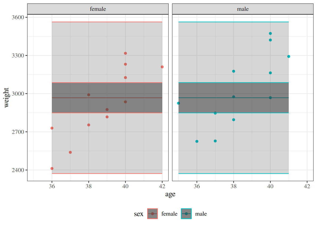
plot_PIs_and_CIs(bw, lm0)

Figure 15: Null model for birthweight data, with 95% confidence and prediction intervals.

This model also has a likelihood:

logLik(lm0)
#> 'log Lik.' -168.955 (df=2)

And we can compare it to more complicated models using a likelihood ratio test:

lrtest(bw_lm2, lm0)

The likelihood ratio statistic for the test comparing the null model to the maximal model is \[\lambda = 2 * (\ell_{\text{full}} - \ell_{0}) = 35.106732\] where:

• \(\ell_{\text{0}}\) is the log-likelihood of the null model: -168.954967
• \(\ell_{\text{full}}\) is the log-likelihood of the maximal model: -151.401601

In R, this test is:

lrtest(lm_max, lm0)

This log-likelihood ratio statistic is called the null deviance. It tells us whether we have enough data to detect a difference between the null and full models.

6.2 Gaussian Deviance vs. GLM Deviance

The residual deviance is a general concept that applies to all GLMs, including Gaussian linear regression. For any GLM, the residual deviance is:

\[D = 2(\ell_{\text{sat}} - \ell(\hat\beta)) \tag{22}\]

where \(\ell_{\text{sat}}\) is the log-likelihood of the saturated model and \(\ell(\hat\beta)\) is the log-likelihood of the fitted model. However, this formula simplifies differently depending on the distribution family, and the resulting test statistics have different null distributions.

Gaussian linear regression deviance

From Equation 8, the Gaussian log-likelihood is:

\[ \ell(\hat\beta, \hat\sigma^2) = -\frac{n}{2}\log(2\pi\hat\sigma^2) - \frac{1}{2\hat\sigma^2} \sum_{i=1}^n(y_i - \hat{y}_i)^2 \]

The saturated model has one free mean parameter per distinct covariate pattern. When there are no replicates (each covariate pattern appears exactly once), it sets \(\hat\mu_i = y_i\) for every observation, so its residual sum of squares is zero:

\[\ell_{\text{sat}}(\hat\sigma^2) = -\frac{n}{2}\log(2\pi\hat\sigma^2)\]

Substituting into Equation 22, the Gaussian deviance simplifies to the residual sum of squares (RSS), scaled by \(\hat\sigma^2\):

\[ D = 2(\ell_{\text{sat}} - \ell(\hat\beta)) = \frac{\sum_{i=1}^n(y_i - \hat{y}_i)^2}{\hat\sigma^2} = \frac{\text{RSS}}{\hat\sigma^2} \]

Because \(\sigma^2\) is unknown and must be estimated, comparing deviances between two nested Gaussian models uses an F-test, which is exact under Gaussian assumptions. Substituting \(D = \text{RSS}/\hat\sigma^2\), the \(\hat\sigma^2\) factors cancel:

\[ F = \frac{(D_1 - D_2) / (p_2 - p_1)}{D_2 / (n - p_2)} = \frac{(\text{RSS}_1 - \text{RSS}_2) / (p_2 - p_1)}{\text{RSS}_2 / (n - p_2)} \ \sim \ F_{p_2 - p_1,\; n - p_2} \]

In R, deviance() applied to an lm object returns RSS (the unscaled deviance):

deviance(bw_lm2)
#> [1] 652425
sum(residuals(bw_lm2)^2)
#> [1] 652425

The two expressions above return the same value.

The Gaussian linear regression model can equivalently be fit as a GLM with family = gaussian, which also returns RSS as the deviance:

bw_glm2 <- glm(
  weight ~ sex + age + sex:age,
  data = bw,
  family = gaussian
)

deviance(bw_lm2)
#> [1] 652425
deviance(bw_glm2)
#> [1] 652425

deviance(bw_lm2) and deviance(bw_glm2) return the same value, confirming that Gaussian linear regression is a special case of the GLM framework where the deviance equals RSS.

Non-Gaussian GLM deviance

For non-Gaussian GLMs, the deviance does not simplify to RSS. The formula depends on the distribution family:

Poisson:

\[ D = 2\sum_{i=1}^n \left[y_i \log\!\left(\frac{y_i}{\hat\mu_i}\right) - (y_i - \hat\mu_i)\right] \]

Binomial:

\[ D = 2\sum_{i=1}^n \left[y_i \log\!\left(\frac{y_i}{\hat\pi_i}\right) + (n_i - y_i)\log\!\left(\frac{n_i - y_i}{n_i - \hat\pi_i}\right)\right] \]

For Poisson and Binomial models, the dispersion parameter \(\phi = 1\) is fixed rather than estimated. Consequently, the difference in deviances between two nested models follows an approximate \(\chi^2\) distribution:

\[D_1 - D_2 \;\dot \sim\; \chi^2_{p_2 - p_1}\]

This asymptotic result replaces the exact F-test used for Gaussian models.

Saturated vs. fully parametrized models with replicates

When some covariate patterns appear more than once (i.e., when there are replicates), it is important to distinguish between two special models:

• The saturated model has one free mean parameter per distinct covariate pattern (\(q\) parameters, where \(q \leq n\) is the number of unique patterns).
• The fully parametrized model has one free mean parameter per observation (\(n\) parameters).

When there are no replicates (\(q = n\)), these two coincide. When there are replicates (\(q < n\)), the saturated model constrains all observations sharing a covariate pattern to have the same mean, but places no constraint on means across different patterns. See Kleinbaum and Klein (2010) for further discussion of this distinction.

Deviance is always measured relative to the saturated model, not the fully parametrized model.

Gaussian deviance with replicates

When covariate pattern \(k\) has \(n_k\) replicates with sample mean \(\bar{y}_k\), the saturated model fits \(\hat\mu_k = \bar{y}_k\) for each pattern \(k\), so its residual sum of squares equals the within-group (pure error) SS:

\[ \text{RSS}_{\text{sat}} = \sum_{k=1}^q \sum_{i: \tilde{x}_i = \tilde{x}_k} (y_i - \bar{y}_k)^2 \]

This is nonzero whenever any covariate pattern has replicates with different response values. The Gaussian deviance relative to the saturated model is therefore:

\[ D = 2(\ell_{\text{sat}} - \ell(\hat\beta)) = \frac{\text{RSS} - \text{RSS}_{\text{sat}}}{\hat\sigma^2} \]

Note

R’s deviance() applied to an lm object returns the total fitted-model RSS, not the deviance relative to the saturated model. To compute the deviance relative to the saturated model, subtract the saturated model’s RSS: deviance(lm_fit) - deviance(lm_saturated).

For the birthweight data, we can verify this directly using bw_lm2 (the interaction model) and lm_max (the saturated model):

deviance(bw_lm2)                      # total RSS of fitted model
#> [1] 652425
deviance(lm_max)                      # within-group (pure error) SS
#> [1] 423783
deviance(bw_lm2) - deviance(lm_max)   # lack-of-fit SS (deviance vs. saturated)
#> [1] 228642

The lack-of-fit SS (deviance(bw_lm2) - deviance(lm_max)) measures how much additional unexplained variation remains after accounting for pure measurement error within covariate patterns.

GLM deviance with replicates

For a Binomial GLM fit to data grouped by covariate pattern (with \(y_k\) events and \(n_k\) observations for pattern \(k\)), the saturated model sets \(\hat\pi_k^{\text{sat}} = y_k / n_k\) for each pattern \(k\). R’s deviance() correctly computes \(2(\ell_{\text{sat}} - \ell(\hat\beta))\) using this grouping:

\[ D = 2\sum_{k=1}^q \left[ y_k \log\!\left(\frac{y_k / n_k}{\hat\pi_k}\right) + (n_k - y_k)\log\!\left(\frac{1 - y_k/n_k}{1 - \hat\pi_k}\right) \right] \]

By convention, terms with \(y_k = 0\) or \(y_k = n_k\) contribute zero to the sum, since \(0\log(0) = 0\) in the limit.

When binomial data is ungrouped (individual Bernoulli observations, \(n_i = 1\)), R uses the fully parametrized model as its reference — assigning \(\hat\pi_i = y_i \in \{0, 1\}\) to each individual observation. Since each predicted probability is exactly 0 or 1, every Bernoulli likelihood contribution equals 1, and hence \(\ell_{\text{fp}} = 0\). Thus R’s deviance() returns \(-2\ell(\hat\beta)\).

We can verify this directly: observations are ungrouped Bernoulli with repeated covariate patterns (\(x \in \{0, 1\}\) appears three times each).

set.seed(42)
x_ug <- rep(0:1, each = 3)
y_ug <- c(0L, 1L, 0L, 1L, 1L, 0L)
fit_ug <- glm(y_ug ~ x_ug, family = binomial)
deviance(fit_ug)                     # R's deviance
#> [1] 7.63817
-2 * as.numeric(logLik(fit_ug))      # -2 * log-likelihood (using ell_fp = 0)
#> [1] 7.63817

The two values are equal, confirming that R uses \(\ell_{\text{fp}} = 0\) as its reference when data are ungrouped.

Note

This reference model is the fully parametrized model (one parameter per observation), not the saturated model (one parameter per distinct covariate pattern). They coincide only when there are no repeated covariate patterns (\(q = n\)). When patterns do repeat (\(q < n\)), the saturated model sets \(\hat\pi_k = y_k/n_k\) per pattern, giving \(\ell_{\text{sat}} < 0\).

deviance() for ungrouped data cannot be used as a goodness-of-fit test against the \(\chi^2\) distribution when \(q < n\). The correct GOF statistic is \(2(\ell_{\text{sat}} - \ell(\hat\beta))\), but R’s deviance() for ungrouped data returns \(-2\ell(\hat\beta)\) (using \(\ell_{\text{fp}} = 0\)). These two quantities differ by \(-2\ell_{\text{sat}} > 0\) whenever \(q < n\). Even if each covariate pattern has many replicates (large \(n_k\)), R’s ungrouped deviance is the wrong statistic to compare against \(\chi^2(q - p)\). To obtain a valid GOF test when patterns repeat, fit the model using grouped data (one row per pattern with \(y_k\) and \(n_k\)), so that R uses the saturated model as its reference.

For further discussion, see Dunn and Smyth (2018, chap. 9) and this Stats Stack Exchange thread.

Summary

Feature	Gaussian linear regression	Non-Gaussian GLMs (e.g., Poisson, Binomial)
Deviance formula	\((\text{RSS} - \text{RSS}_{\text{sat}})/\hat\sigma^2\)	\(2(\ell_{\text{sat}} - \ell(\hat\beta))\)
deviance() in R	Returns total RSS	Returns \(2(\ell_{\text{sat}} - \ell(\hat\beta))\)
Saturated model reference	Per covariate pattern	Per covariate pattern (grouped) or per observation (ungrouped)
Dispersion \(\phi\)	Unknown; estimated as \(s^2 = \text{RSS}/(n-p)\)	Fixed (\(\phi = 1\))
Test for nested models	F-test (exact)	\(\chi^2\)-test (asymptotic)

6.3 Diagnostics

Tip

This section is adapted from Dobson and Barnett (2018, secs. 6.2–6.3) and Dunn and Smyth (2018) Chapter 3.

Assumptions in linear regression models

\[Y_i|\tilde{X}_i \sim_{{\color{red}\perp\!\!\!\perp}} {\color{blue}\text{N}}({\color{orange}\mu_i}, {\color{green}\sigma^2})\] \[{\color{orange}\mu_i = \tilde{x}\cdot \tilde{\beta}}\]

1. \({\color{blue}\text{Normality}}\)

The model assumes that the distribution conditional on a given \(X\) value is Gaussian.

2. \({\color{orange}\text{Correct Functional Form}}\) of Conditional Mean Structure (Linear Component)

The model assumes that the conditional means have the structure: \[\text{E}[Y|\tilde{X}= \tilde{x}] = \tilde{x}'\tilde{\beta}\]

3. \({\color{green}\text{Homoskedasticity}}\)

The model assumes that variance \(\sigma^2\) is constant (with respect to \(\tilde{x}\)).

4. \({\color{red}\text{Independence}}\)

The model assumes that the observations are statistically independent.

Direct visualization

The most direct way to examine the fit of a model is to compare it to the raw observed data.

bw <-
  bw |>
  mutate(
    predlm2 = predict(bw_lm2)
  ) |>
  arrange(sex, age)

plot1_interact <-
  plot1 %+% bw +
  geom_line(aes(y = predlm2))

print(plot1_interact)

Figure 16: Birthweight model with interaction term

It’s not easy to assess these assumptions from this model. If there are multiple continuous covariates, it becomes even harder to visualize the raw data.

Fitted model for hers data

Consider the hers data from Vittinghoff et al. (2012).

The “heart and estrogen/progestin study” (HERS) was a clinical trial of hormone therapy for prevention of recurrent heart attacks and death among 2,763 post-menopausal women with existing coronary heart disease (CHD) (Hulley et al. 1998).

hers <- fs::path_package("rme", "extdata/hersdata.dta") |> 
  haven::read_dta()
hers

Table 28: hers data

Suppose we consider models with and without intercept terms (i.e., possibly forcing the intercept to go through 0):

hers_lm_with_int <- lm(
  na.action = na.exclude,
  LDL ~ smoking * age, data = hers
)


library(equatiomatic)
equatiomatic::extract_eq(hers_lm_with_int)

\[ \operatorname{LDL} = \alpha + \beta_{1}(\operatorname{smoking}) + \beta_{2}(\operatorname{age}) + \beta_{3}(\operatorname{smoking} \times \operatorname{age}) + \epsilon \]

hers_lm_no_int <- lm(
  na.action = na.exclude,
  LDL ~ age + smoking:age - 1, data = hers
)

library(equatiomatic)
equatiomatic::extract_eq(hers_lm_no_int)

\[ \operatorname{LDL} = \beta_{1}(\operatorname{age}) + \beta_{2}(\operatorname{age} \times \operatorname{age}_{\operatorname{smoking}}) + \epsilon \]

Table 29: hers data models with and without intercepts

library(gtsummary)
hers_lm_with_int |> 
  tbl_regression(intercept = TRUE)

(a) With intercept

Characteristic	Beta	95% CI	p-value
(Intercept)	154	138, 170	<0.001
current smoker	54	15, 94	0.007
age in years	-0.14	-0.38, 0.09	0.2
current smoker * age in years	-0.79	-1.4, -0.17	0.012
Abbreviation: CI = Confidence Interval

hers_lm_no_int |> 
  tbl_regression(intercept = TRUE)

(b) No intercept

Characteristic	Beta	95% CI	p-value
age in years	2.1	2.1, 2.2	<0.001
age in years * current smoker	0.19	0.12, 0.26	<0.001
Abbreviation: CI = Confidence Interval

Figure 17: hers data models with and without intercepts

library(sjPlot)

hers_plot1 <- hers_lm_no_int |>
  sjPlot::plot_model(
    type = "pred",
    terms = c("age", "smoking"),
    show.data = TRUE
  ) +
  facet_wrap(~group_col, ncol = 1) +
  expand_limits(y = 0) +
  theme(legend.position = "bottom")

hers_plot1

(a) No intercept

library(sjPlot)

hers_plot2 <- hers_lm_with_int |>
  sjPlot::plot_model(
    type = "pred",
    terms = c("age", "smoking"),
    show.data = TRUE
  ) +
  facet_wrap(~group_col, ncol = 1) +
  expand_limits(y = 0) +
  theme(legend.position = "bottom")

hers_plot2

(b) With intercept

Residuals

Maybe we can transform the data and model in some way to make it easier to inspect.

Definition 6 (Residual noise/deviation from the population mean) The residual noise in a probabilistic model \(p(Y)\), also known as the residual deviation of an observation from its population mean or residual for short, is the difference between an observed value \(y\) and its population mean:

\[\varepsilon(y) \stackrel{\text{def}}{=}y - \text{E}{\left[Y\right]} \tag{23}\]

We use the same notation for residual noise that we used for errors.

\(\text{E}{\left[Y\right]}\) can be viewed as an estimate of \(Y\), before \(y\) is observed. Conversely, each observation \(y\) can be viewed as an estimate of \(\text{E}{\left[Y\right]}\) (albeit an imprecise one, individually, since \(n=1\)).

We can rearrange Equation 23 to view \(y\) as the sum of its mean plus the residual noise:

\[y = \text{E}{\left[Y\right]} + \varepsilon{\left(y\right)}\]

Theorem 3 (Residuals in Gaussian models) If \(Y\) has a Gaussian distribution, then \(\varepsilon(Y)\) also has a Gaussian distribution, and vice versa.

Proof. Left to the reader.

Definition 7 (Residuals of a fitted model value) The residual of a fitted value \(\hat y\) (shorthand: “residual”) is its error relative to the observed data: \[ \begin{aligned} e(\hat y) &\stackrel{\text{def}}{=}\varepsilon{\left(\hat y\right)} \\&= y - \hat y \end{aligned} \]

Example 4 (residuals in birthweight data)  

plot1_interact +
  facet_wrap(~sex) +
  geom_segment(
    aes(
      x = age,
      y = predlm2,
      xend = age,
      yend = weight,
      col = sex,
      group = id
    ),
    linetype = "dotted"
  )

Figure 18: Fitted values and residuals for interaction model for birthweight data

Residuals of fitted values vs residual noise

\(e(\hat y)\) can be seen as the maximum likelihood estimate of the residual noise:

\[ \begin{aligned} e(\hat y) &= y - \hat y \\ &= \hat\varepsilon_{ML} \end{aligned} \]

General characteristics of residuals

Theorem 4 If \(\hat{\text{E}}{\left[Y\right]}\) is an unbiased estimator of the mean \(\text{E}{\left[Y\right]}\), then:

\[\text{E}{\left[e(y)\right]} = 0 \tag{24}\] \[\text{Var}{\left(e(y)\right)} \approx \sigma^2 \tag{25}\]

Proof.  

Equation 24:

\[ \begin{aligned} \text{E}{\left[e(y)\right]} &= \text{E}{\left[y - \hat y\right]} \\ &= \text{E}{\left[y\right]} - \text{E}{\left[\hat y\right]} \\ &= \text{E}{\left[y\right]} - \text{E}{\left[y\right]} \\ &= 0 \end{aligned} \]

Equation 25:

\[ \begin{aligned} \text{Var}{\left(e(y)\right)} &= \text{Var}{\left(y - \hat y\right)} \\ &= \text{Var}{\left(y\right)} + \text{Var}{\left(\hat y\right)} - 2 \text{Cov}{\left(y, \hat y\right)} \\ &{\dot{\approx}} \text{Var}{\left(y\right)} + 0 - 2 \cdot 0 \\ &= \text{Var}{\left(y\right)} \\ &= \sigma^2 \end{aligned} \]

Characteristics of residuals in Gaussian models

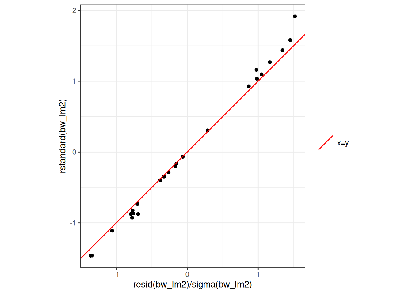
With enough data and a correct model, the residuals will be approximately Gaussian distributed, with variance \(\sigma^2\), which we can estimate using \(\hat\sigma^2\); that is:

\[ e_i \ \sim_{\text{iid}}\ N(0, \hat\sigma^2) \]

Computing residuals in R

R provides a function for residuals:

resid(bw_lm2)
#>         1         2         3         4         5         6         7         8 
#>  176.2667 -140.7333 -144.1333  -59.5333  177.4667 -126.9333  -68.9333  242.6667 
#>         9        10        11        12        13        14        15        16 
#> -139.3333   51.6667  156.6667 -125.1333  274.2759 -137.7069  -27.6897 -246.6897 
#>        17        18        19        20        21        22        23        24 
#> -191.6724  189.3276  -11.6724 -242.6379  -47.6379  262.3621  210.3621  -30.6207

Exercise 20 Check R’s output by computing the residuals directly.

Solution.  

bw$weight - fitted(bw_lm2)
#>         1         2         3         4         5         6         7         8 
#>  176.2667 -140.7333 -144.1333  -59.5333  177.4667 -126.9333  -68.9333  242.6667 
#>         9        10        11        12        13        14        15        16 
#> -139.3333   51.6667  156.6667 -125.1333  274.2759 -137.7069  -27.6897 -246.6897 
#>        17        18        19        20        21        22        23        24 
#> -191.6724  189.3276  -11.6724 -242.6379  -47.6379  262.3621  210.3621  -30.6207

This matches R’s output!

Graphing the residuals

Figure 19: Fitted values and residuals for interaction model for birthweight data

plot1_interact +
  facet_wrap(~sex) +
  geom_segment(
    aes(
      x = age,
      y = predlm2,
      xend = age,
      yend = weight,
      col = sex,
      group = id
    ),
    linetype = "dotted"
  )

(a) fitted values

bw <- bw |>
  mutate(
    resids_intxn =
      weight - fitted(bw_lm2)
  )

plot_bw_resid <-
  bw |>
  ggplot(aes(
    x = age,
    y = resids_intxn,
    linetype = sex,
    shape = sex,
    col = sex
  )) +
  theme_bw() +
  xlab("Gestational age (weeks)") +
  ylab("residuals (grams)") +
  theme(legend.position = "bottom") +
  geom_hline(aes(
    yintercept = 0,
    col = sex
  )) +
  geom_segment(
    aes(yend = 0),
    linetype = "dotted"
  ) +
  geom_point()
# expand_limits(y = 0, x = 0) +
geom_point(alpha = .7)
#> geom_point: na.rm = FALSE
#> stat_identity: na.rm = FALSE
#> position_identity
print(plot_bw_resid + facet_wrap(~sex))

(b) Residuals

Residuals versus predictors

hers <- hers |>
  mutate(
    resids_no_intcpt =
      LDL - fitted(hers_lm_no_int),
    resids_with_intcpt =
      LDL - fitted(hers_lm_with_int)
  )

Figure 20: Residuals of hers data vs predictors

hers |>
  arrange(age) |>
  ggplot() +
  aes(x = age, y = resids_no_intcpt, col = factor(smoking)) +
  geom_point() +
  geom_hline(aes(yintercept = 0, col = factor(smoking))) +
  facet_wrap(~smoking, labeller = "label_both") +
  theme(legend.position = "bottom") +
  geom_smooth(col = "blue")

(a) no intercept

hers |>
  arrange(age) |>
  ggplot() +
  aes(x = age, y = resids_with_intcpt, col = factor(smoking)) +
  geom_point() +
  geom_hline(aes(yintercept = 0, col = factor(smoking))) +
  facet_wrap(~smoking, labeller = "label_both") +
  theme(legend.position = "bottom") +
  geom_smooth(col = "blue")

(b) with intercept

Residuals versus fitted values

If the model contains multiple continuous covariates, how do we check for errors in the mean structure assumption?

library(ggfortify)
hers_lm_no_int |>
  update(na.action = na.omit) |>
  autoplot(
    which = 1,
    ncol = 1,
    smooth.colour = NA
  ) +
  geom_hline(yintercept = 0, col = "red")

Figure 21: Residuals of interaction model for hers data

We can add a LOESS smooth to visualize where the residual mean is nonzero:

library(ggfortify)
hers_lm_no_int |>
  update(na.action = na.omit) |>
  autoplot(
    which = 1,
    ncol = 1
  ) +
  geom_hline(yintercept = 0, col = "red")

Figure 22: Residuals of interaction model for hers data, no intercept term

Figure 23: Residuals of interaction model for hers data, with and without intercept term

library(ggfortify)
hers_lm_no_int |>
  update(na.action = na.omit) |>
  autoplot(
    which = 1,
    ncol = 1
  ) +
  geom_hline(yintercept = 0, col = "red")

(a) no intercept term

hers_lm_with_int |>
  update(na.action = na.omit) |>
  autoplot(
    which = 1,
    ncol = 1
  ) +
  geom_hline(yintercept = 0, col = "red")

(b) with intercept term

Definition 8 (Standardized residuals) \[r_i = \frac{e_i}{\widehat{SD}(e_i)}\]

Hence, with enough data and a correct model, the standardized residuals will be approximately standard Gaussian; that is,

\[ r_i \ \sim_{\text{iid}}\ N(0,1) \]

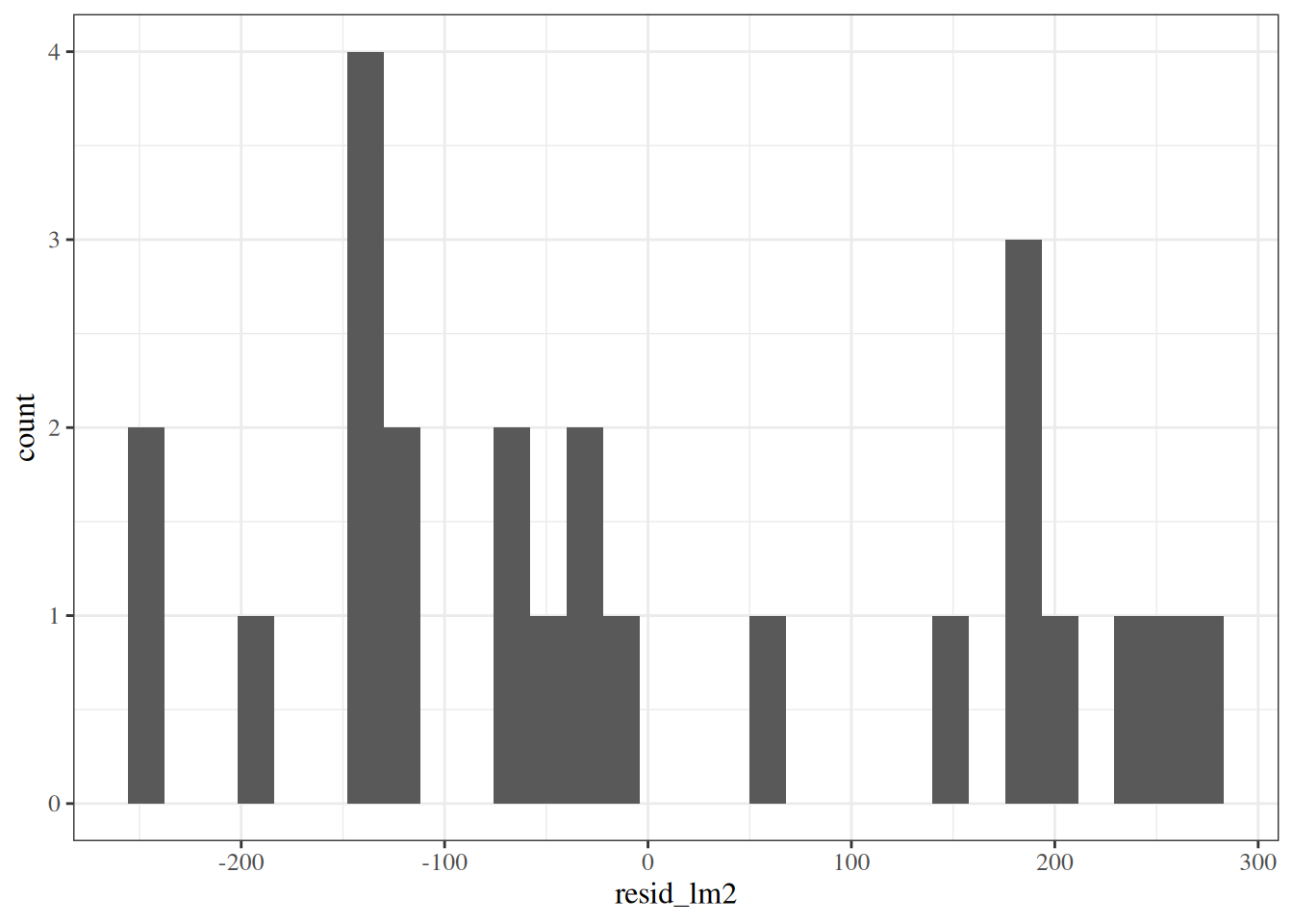
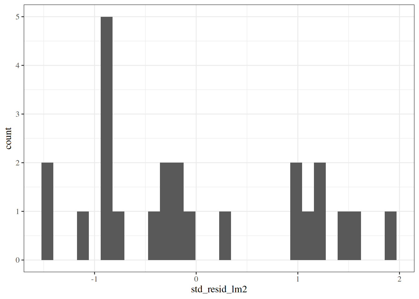
Marginal distributions of residuals

To look for problems with our model, we can check whether the residuals \(e_i\) and standardized residuals \(r_i\) look like they have the distributions that they are supposed to have, according to the model.

Standardized residuals in R

rstandard(bw_lm2)
#>          1          2          3          4          5          6          7 
#>  1.1598166 -0.9260109 -0.8747917 -0.3472255  1.0350665 -0.7347315 -0.3990086 
#>          8          9         10         11         12         13         14 
#>  1.4375164 -0.8253872  0.3060646  0.9280669 -0.8761592  1.9142780 -0.8655921 
#>         15         16         17         18         19         20         21 
#> -0.1642993 -1.4637574 -1.1101599  1.0965787 -0.0676062 -1.4615865 -0.2869582 
#>         22         23         24 
#>  1.5803994  1.2671652 -0.1980543
resid(bw_lm2) / sigma(bw_lm2)
#>          1          2          3          4          5          6          7 
#>  0.9759331 -0.7791962 -0.7980209 -0.3296173  0.9825771 -0.7027900 -0.3816622 
#>          8          9         10         11         12         13         14 
#>  1.3435690 -0.7714449  0.2860621  0.8674141 -0.6928239  1.5185792 -0.7624398 
#>         15         16         17         18         19         20         21 
#> -0.1533089 -1.3658431 -1.0612299  1.0482473 -0.0646265 -1.3434099 -0.2637562 
#>         22         23         24 
#>  1.4526163  1.1647086 -0.1695371

These are not quite the same, because R is doing something more complicated and precise to get the standard errors. Let’s not worry about those details for now; the difference is pretty small in this case:

rstandard_compare_plot <-
  tibble(
    x = resid(bw_lm2) / sigma(bw_lm2),
    y = rstandard(bw_lm2)
  ) |>
  ggplot(aes(x = x, y = y)) +
  geom_point() +
  theme_bw() +
  coord_equal() +
  xlab("resid(bw_lm2)/sigma(bw_lm2)") +
  ylab("rstandard(bw_lm2)") +
  geom_abline(
    aes(
      intercept = 0,
      slope = 1,
      col = "x=y"
    )
  ) +
  labs(colour = "") +
  scale_colour_manual(values = "red")

print(rstandard_compare_plot)

Let’s add these residuals to the tibble of our dataset:

bw <-
  bw |>
  mutate(
    fitted_lm2 = fitted(bw_lm2),
    resid_lm2 = resid(bw_lm2),
    resid_lm2_alt = weight - fitted_lm2,
    std_resid_lm2 = rstandard(bw_lm2),
    std_resid_lm2_alt = resid_lm2 / sigma(bw_lm2)
  )

bw |>
  select(
    sex,
    age,
    weight,
    fitted_lm2,
    resid_lm2,
    std_resid_lm2
  )

Now let’s build histograms:

resid_marginal_hist <-
  bw |>
  ggplot(aes(x = resid_lm2)) +
  geom_histogram()

print(resid_marginal_hist)

Figure 24: Marginal distribution of (nonstandardized) residuals

Hard to tell with this small amount of data, but I’m a bit concerned that the histogram doesn’t show a bell-curve shape.

std_resid_marginal_hist <-
  bw |>
  ggplot(aes(x = std_resid_lm2)) +
  geom_histogram()

print(std_resid_marginal_hist)

Figure 25: Marginal distribution of standardized residuals

This looks similar, although the scale of the x-axis got narrower, because we divided by \(\hat\sigma\) (roughly speaking).

Still hard to tell if the distribution is Gaussian.

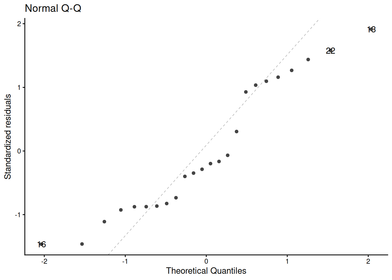
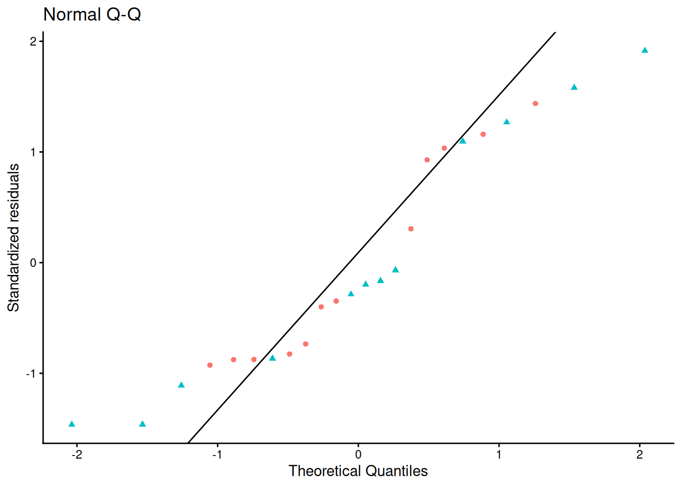
QQ plot of standardized residuals

Another way to assess normality is the QQ plot of the standardized residuals versus normal quantiles:

library(ggfortify)
# needed to make ggplot2::autoplot() work for `lm` objects

qqplot_lm2_auto <-
  bw_lm2 |>
  autoplot(
    which = 2, # options are 1:6; can do multiple at once
    ncol = 1
  ) +
  theme_classic()

print(qqplot_lm2_auto)

If the Gaussian model were correct, these points should follow the dotted line.

Fig 2.4 panel (c) in Dobson and Barnett (2018) is a little different; they didn’t specify how they produced it, but other statistical analysis systems do things differently from R.

See also Dunn and Smyth (2018) §3.5.4.

QQ plot - how it’s built

Let’s construct it by hand:

bw <- bw |>
  mutate(
    p = (rank(std_resid_lm2) - 1 / 2) / n(), # "Blom's method"
    expected_quantiles_lm2 = qnorm(p)
  )

qqplot_lm2 <-
  bw |>
  ggplot(
    aes(
      x = expected_quantiles_lm2,
      y = std_resid_lm2,
      col = sex,
      shape = sex
    )
  ) +
  geom_point() +
  theme_classic() +
  theme(legend.position = "none") + # removing the plot legend
  ggtitle("Normal Q-Q") +
  xlab("Theoretical Quantiles") +
  ylab("Standardized residuals")

# find the expected line:

ps <- c(.25, .75) # reference probabilities
a <- quantile(rstandard(bw_lm2), ps) # empirical quantiles
b <- qnorm(ps) # theoretical quantiles

qq_slope <- diff(a) / diff(b)
qq_intcpt <- a[1] - b[1] * qq_slope

qqplot_lm2 <-
  qqplot_lm2 +
  geom_abline(slope = qq_slope, intercept = qq_intcpt)

print(qqplot_lm2)

Conditional distributions of residuals

If our Gaussian linear regression model is correct, the residuals \(e_i\) and standardized residuals \(r_i\) should have:

• an approximately Gaussian distribution, with:
• a mean of 0
• a constant variance

This should be true for every value of \(x\).

If we didn’t correctly guess the functional form of the linear component of the mean, \[\text{E}[Y|X=x] = \beta_0 + \beta_1 X_1 + ... + \beta_p X_p\]

Then the residuals might have nonzero mean.

Regardless of whether we guessed the mean function correctly, ther the variance of the residuals might differ between values of \(x\).

Residuals versus fitted values

To look for these issues, we can plot the residuals \(e_i\) against the fitted values \(\hat y_i\) (Figure 26).

autoplot(bw_lm2, which = 1, ncol = 1) |> print()

Figure 26: birthweight model (Equation 3): residuals versus fitted values

If the model is correct, the blue line should stay flat and close to 0, and the cloud of dots should have the same vertical spread regardless of the fitted value.

If not, we probably need to change the functional form of linear component of the mean, \[\text{E}[Y|X=x] = \beta_0 + \beta_1 X_1 + ... + \beta_p X_p\]

Example: PLOS Medicine title length data

(Adapted from Dobson and Barnett (2018), §6.7.1)

data(PLOS, package = "dobson")
library(ggplot2)
fig1 = 
  PLOS |> 
  ggplot(
    aes(x = authors,
        y = nchar)
  ) +
  geom_point() +
  theme(legend.position = "bottom") +
  labs(col = "") +
  guides(col=guide_legend(ncol=3))
fig1

Figure 27: Number of authors versus title length in PLOS Medicine articles

Linear fit

lm_PLOS_linear = lm(
  formula = nchar ~ authors, 
  data = PLOS)

fig2 = fig1 +
  geom_smooth(
    method = "lm", 
              fullrange = TRUE,
              aes(col = "lm(y ~ x)"))
fig2

library(ggfortify)
autoplot(lm_PLOS_linear, which = 1, ncol = 1)

Figure 28: Number of authors versus title length in PLOS Medicine, with linear model fit

(a) Data and fit

(b) Residuals vs fitted

Quadratic fit

lm_PLOS_quad = lm(
  formula = nchar ~ authors + I(authors^2), 
  data = PLOS)

fig3 = 
  fig2 + 
geom_smooth(
    method = "lm",
    fullrange = TRUE,
    formula = y ~ x + I(x ^ 2),
    aes(col = "lm(y ~ x + I(x^2))")
  )
fig3

autoplot(lm_PLOS_quad, which = 1, ncol = 1)

Figure 29: Number of authors versus title length in PLOS Medicine, with quadratic model fit

(a) Data and fit

(b) Residuals vs fitted

Linear versus quadratic fits

library(ggfortify)
autoplot(lm_PLOS_linear, which = 1, ncol = 1)

autoplot(lm_PLOS_quad, which = 1, ncol = 1)

Figure 30: Residuals versus fitted plot for linear and quadratic fits to PLOS data

(a) Linear

(b) Quadratic

Cubic fit

lm_PLOS_cub = lm(
  formula = nchar ~ authors + I(authors^2) + I(authors^3), 
  data = PLOS)

fig4 = 
  fig3 + 
geom_smooth(
    method = "lm",
    fullrange = TRUE,
    formula = y ~ x + I(x ^ 2) + I(x ^ 3),
    aes(col = "lm(y ~ x + I(x^2) + I(x ^ 3))")
  )
fig4

autoplot(lm_PLOS_cub, which = 1, ncol = 1)

Figure 31: Number of authors versus title length in PLOS Medicine, with cubic model fit

(a) Data and fit

(b) Residuals vs fitted

Logarithmic fit

lm_PLOS_log = lm(nchar ~ log(authors), data = PLOS)

fig5 = fig4 + 
  geom_smooth(
    method = "lm",
    fullrange = TRUE,
    formula = y ~ log(x),
    aes(col = "lm(y ~ log(x))")
  )
fig5

autoplot(lm_PLOS_log, which = 1, ncol = 1)

Figure 32: logarithmic fit

(a) Data and fit

(b) Residuals vs fitted

Model selection

anova(lm_PLOS_linear, lm_PLOS_quad)

Table 30: linear vs quadratic

anova(lm_PLOS_quad, lm_PLOS_cub)

Table 31: quadratic vs cubic

AIC/BIC

AIC(lm_PLOS_quad)
#> [1] 8567.61
AIC(lm_PLOS_cub)
#> [1] 8554.51

AIC(lm_PLOS_cub)
#> [1] 8554.51
AIC(lm_PLOS_log)
#> [1] 8543.63

BIC(lm_PLOS_cub)
#> [1] 8578.4
BIC(lm_PLOS_log)
#> [1] 8557.97

Extrapolation is dangerous

fig_all = fig5 +
  xlim(0, 60)
fig_all

Figure 33: Number of authors versus title length in PLOS Medicine

Scale-location plot

We can also plot the square roots of the absolute values of the standardized residuals against the fitted values (Figure 34).

autoplot(bw_lm2, which = 3, ncol = 1) |> print()

Figure 34: Scale-location plot of birthweight data

Here, the blue line doesn’t need to be near 0, but it should be flat. If not, the residual variance \(\sigma^2\) might not be constant, and we might need to transform our outcome \(Y\) (or use a model that allows non-constant variance).

Residuals versus leverage

We can also plot our standardized residuals against “leverage”, which roughly speaking is a measure of how unusual each \(x_i\) value is. Very unusual \(x_i\) values can have extreme effects on the model fit, so we might want to remove those observations as outliers, particularly if they have large residuals.

autoplot(bw_lm2, which = 5, ncol = 1) |> print()

Figure 35: birthweight model with interactions (Equation 3): residuals versus leverage

The blue line should be relatively flat and close to 0 here.

Diagnostics constructed by hand

bw <-
  bw |>
  mutate(
    predlm2 = predict(bw_lm2),
    residlm2 = weight - predlm2,
    std_resid = residlm2 / sigma(bw_lm2),
    # std_resid_builtin = rstandard(bw_lm2), # uses leverage
    sqrt_abs_std_resid = std_resid |> abs() |> sqrt()
  )

Residuals vs fitted

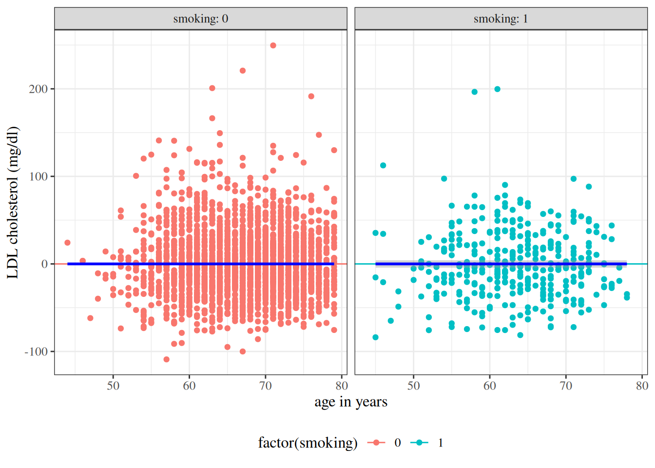
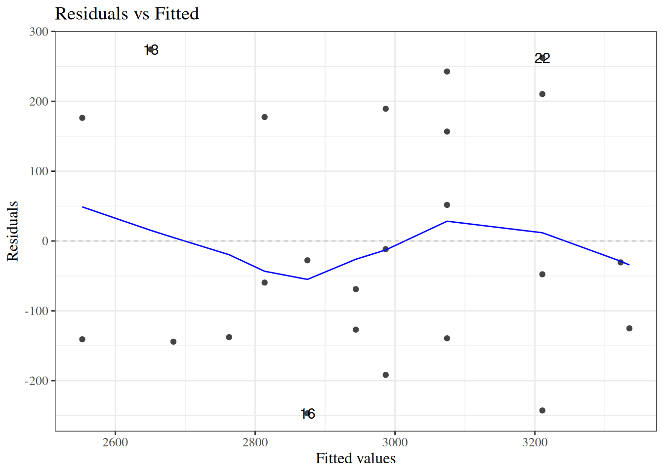
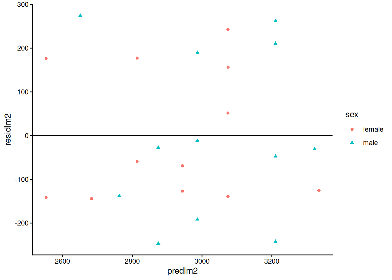
resid_vs_fit <- bw |>
  ggplot(
    aes(x = predlm2, y = residlm2, col = sex, shape = sex)
  ) +
  geom_point() +
  theme_classic() +
  geom_hline(yintercept = 0)

print(resid_vs_fit)

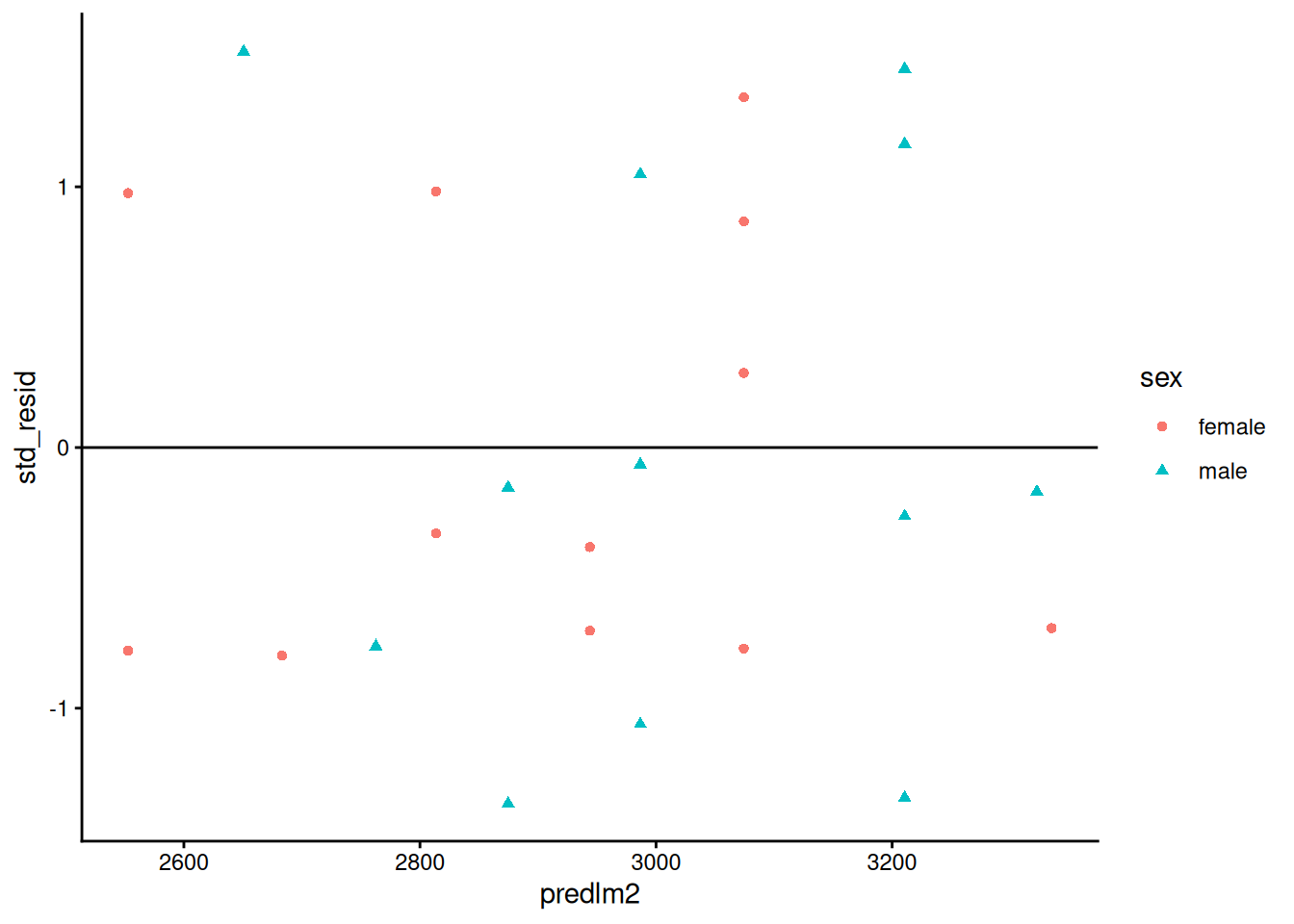
Standardized residuals vs fitted

bw |>
  ggplot(
    aes(x = predlm2, y = std_resid, col = sex, shape = sex)
  ) +
  geom_point() +
  theme_classic() +
  geom_hline(yintercept = 0)

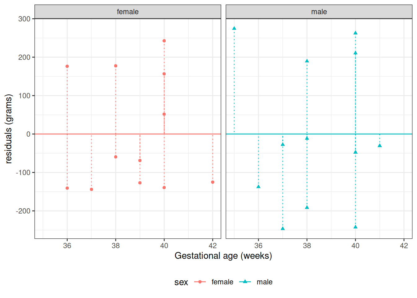
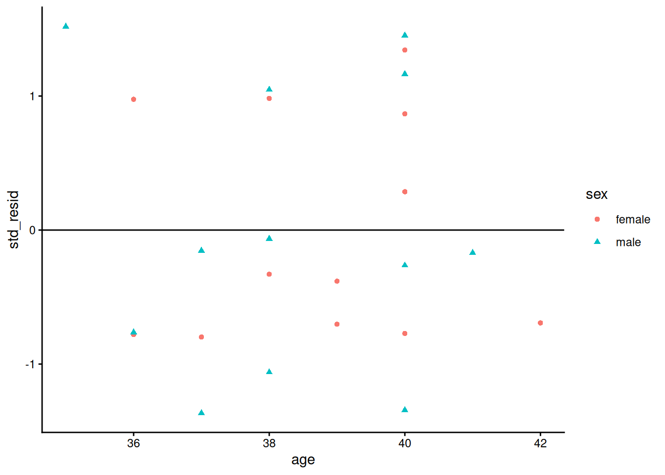
Standardized residuals vs gestational age

bw |>
  ggplot(
    aes(x = age, y = std_resid, col = sex, shape = sex)
  ) +
  geom_point() +
  theme_classic() +
  geom_hline(yintercept = 0)

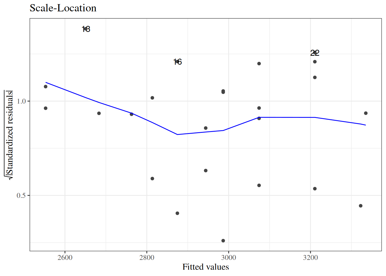
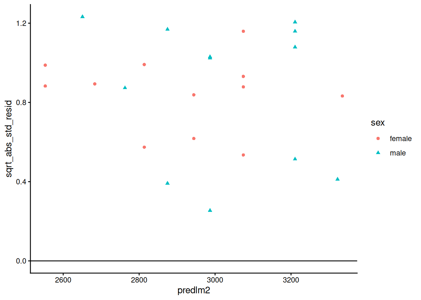
sqrt(abs(rstandard())) vs fitted

Compare with autoplot(bw_lm2, 3)

bw |>
  ggplot(
    aes(x = predlm2, y = sqrt_abs_std_resid, col = sex, shape = sex)
  ) +
  geom_point() +
  theme_classic() +
  geom_hline(yintercept = 0)

6.4 Model selection

(adapted from Dobson and Barnett (2018) §6.3.3; for more information on prediction, see James et al. (2013) and Harrell (2015)).

If we have a lot of covariates in our dataset, we might want to choose a small subset to use in our model.

There are a few possible metrics to consider for choosing a “best” model.

Mean squared error

We might want to minimize the mean squared error, \(\text E[(y-\hat y)^2]\), for new observations that weren’t in our data set when we fit the model.

Unfortunately, \[\frac{1}{n}\sum_{i=1}^n (y_i-\hat y_i)^2\] gives a biased estimate of \(\text E[(y-\hat y)^2]\) for new data. If we want an unbiased estimate, we will have to be clever.

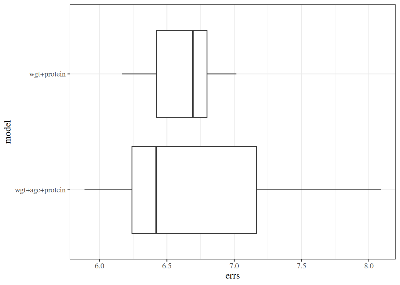
Cross-validation

data("carbohydrate", package = "dobson")
library(cvTools)
full_model <- lm(carbohydrate ~ ., data = carbohydrate)
cv_full <-
  full_model |> cvFit(
    data = carbohydrate, K = 5, R = 10,
    y = carbohydrate$carbohydrate
  )

reduced_model <- full_model |> update(formula = ~ . - age)

cv_reduced <-
  reduced_model |> cvFit(
    data = carbohydrate, K = 5, R = 10,
    y = carbohydrate$carbohydrate
  )

results_reduced <-
  tibble(
    model = "wgt+protein",
    errs = cv_reduced$reps[]
  )
results_full <-
  tibble(
    model = "wgt+age+protein",
    errs = cv_full$reps[]
  )

cv_results <-
  bind_rows(results_reduced, results_full)

cv_results |>
  ggplot(aes(y = model, x = errs)) +
  geom_boxplot()

comparing metrics

compare_results <- tribble(
  ~model, ~cvRMSE, ~r.squared, ~adj.r.squared, ~trainRMSE, ~loglik,
  "full",
  cv_full$cv,
  summary(full_model)$r.squared,
  summary(full_model)$adj.r.squared,
  sigma(full_model),
  logLik(full_model) |> as.numeric(),
  "reduced",
  cv_reduced$cv,
  summary(reduced_model)$r.squared,
  summary(reduced_model)$adj.r.squared,
  sigma(reduced_model),
  logLik(reduced_model) |> as.numeric()
)

compare_results

anova(full_model, reduced_model)

stepwise regression

Caution about stepwise selection

Stepwise regression has several known problems:

• It tends to select too many variables (overfitting)
• P-values and confidence intervals are biased after selection
• It ignores model uncertainty
• Results can be unstable across different samples

Consider using cross-validation, penalized methods (like Lasso), or subject-matter knowledge instead. See Harrell (2015) and Heinze et al. (2018) for more discussion.

library(olsrr)
olsrr:::ols_step_both_aic(full_model)
#> 
#> 
#>                              Stepwise Summary                              
#> -------------------------------------------------------------------------
#> Step    Variable         AIC        SBC       SBIC       R2       Adj. R2 
#> -------------------------------------------------------------------------
#>  0      Base Model     140.773    142.764    83.068    0.00000    0.00000 
#>  1      protein (+)    137.950    140.937    80.438    0.21427    0.17061 
#>  2      weight (+)     132.981    136.964    77.191    0.44544    0.38020 
#> -------------------------------------------------------------------------
#> 
#> Final Model Output 
#> ------------------
#> 
#>                          Model Summary                          
#> ---------------------------------------------------------------
#> R                       0.667       RMSE                 5.505 
#> R-Squared               0.445       MSE                 30.301 
#> Adj. R-Squared          0.380       Coef. Var           15.879 
#> Pred R-Squared          0.236       AIC                132.981 
#> MAE                     4.593       SBC                136.964 
#> ---------------------------------------------------------------
#>  RMSE: Root Mean Square Error 
#>  MSE: Mean Square Error 
#>  MAE: Mean Absolute Error 
#>  AIC: Akaike Information Criteria 
#>  SBC: Schwarz Bayesian Criteria 
#> 
#>                                ANOVA                                
#> -------------------------------------------------------------------
#>                 Sum of                                             
#>                Squares        DF    Mean Square      F        Sig. 
#> -------------------------------------------------------------------
#> Regression     486.778         2        243.389    6.827    0.0067 
#> Residual       606.022        17         35.648                    
#> Total         1092.800        19                                   
#> -------------------------------------------------------------------
#> 
#>                                   Parameter Estimates                                    
#> ----------------------------------------------------------------------------------------
#>       model      Beta    Std. Error    Std. Beta      t        Sig      lower     upper 
#> ----------------------------------------------------------------------------------------
#> (Intercept)    33.130        12.572                  2.635    0.017     6.607    59.654 
#>     protein     1.824         0.623        0.534     2.927    0.009     0.509     3.139 
#>      weight    -0.222         0.083       -0.486    -2.662    0.016    -0.397    -0.046 
#> ----------------------------------------------------------------------------------------

Lasso

\[\arg \max_{\theta} {\left\{\ell(\theta) - \lambda \sum_{j=1}^p|\beta_j|\right\}}\]

library(glmnet)
y <- carbohydrate$carbohydrate
x <- carbohydrate |>
  select(age, weight, protein) |>
  as.matrix()
fit <- glmnet(x, y)

autoplot(fit, xvar = "lambda")

Figure 36: Lasso selection

cvfit <- cv.glmnet(x, y)
plot(cvfit)

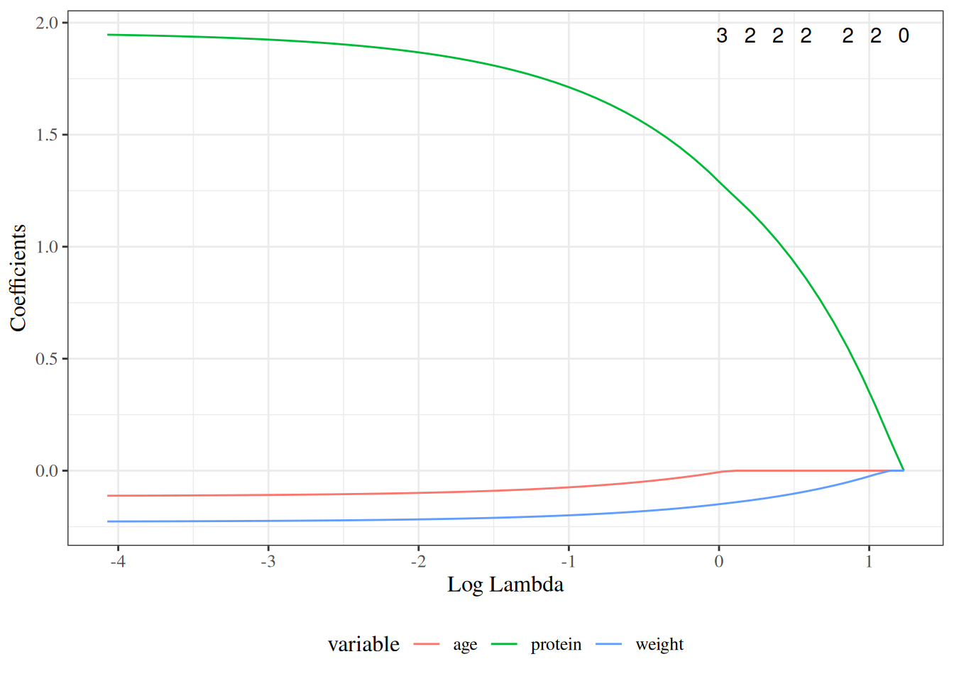
coef(cvfit, s = "lambda.1se")
#> 4 x 1 sparse Matrix of class "dgCMatrix"
#>             lambda.1se
#> (Intercept) 34.3091615
#> age          .        
#> weight      -0.0800142
#> protein      0.7640510

Akaike, Hirotugu. 1974. “A New Look at the Statistical Model Identification.” IEEE Transactions on Automatic Control 19 (6): 716–23. https://doi.org/10.1109/TAC.1974.1100705.

Anderson, Edgar. 1935. “The Irises of the Gaspe Peninsula.” Bulletin of American Iris Society 59: 2–5.

Chatterjee, Samprit, and Ali S Hadi. 2015. Regression Analysis by Example. John Wiley & Sons. https://www.wiley.com/en-us/Regression+Analysis+by+Example%2C+4th+Edition-p-9780470055458.

Dobson, Annette J, and Adrian G Barnett. 2018. An Introduction to Generalized Linear Models. 4th ed. CRC press. https://doi.org/10.1201/9781315182780.

Dunn, Peter K, and Gordon K Smyth. 2018. Generalized Linear Models with Examples in R. Vol. 53. Springer. https://link.springer.com/book/10.1007/978-1-4419-0118-7.

Faraway, Julian J. 2025. Linear Models with R. https://www.routledge.com/Linear-Models-with-R/Faraway/p/book/9781032583983.

Harrell, Frank E. 2015. Regression Modeling Strategies: With Applications to Linear Models, Logistic Regression, and Survival Analysis. 2nd ed. Springer. https://doi.org/10.1007/978-3-319-19425-7.

Heinze, Georg, Christine Wallisch, and Daniela Dunkler. 2018. “Variable Selection – A Review and Recommendations for the Practicing Statistician.” Biometrical Journal 60 (3): 431–49. https://doi.org/10.1002/bimj.201700067.

Hogg, Robert V., Elliot A. Tanis, and Dale L. Zimmerman. 2015. Probability and Statistical Inference. Ninth edition. Pearson.

Hulley, Stephen, Deborah Grady, Trudy Bush, et al. 1998. “Randomized Trial of Estrogen Plus Progestin for Secondary Prevention of Coronary Heart Disease in Postmenopausal Women.” JAMA : The Journal of the American Medical Association (Chicago, IL) 280 (7): 605–13.

James, Gareth, Daniela Witten, Trevor Hastie, Robert Tibshirani, et al. 2013. An Introduction to Statistical Learning. Vol. 112. Springer. https://www.statlearning.com/.

Kleinbaum, David G, and Mitchel Klein. 2010. Logistic Regression: A Self-Learning Text. 3rd ed. Springer. https://link.springer.com/book/10.1007/978-1-4419-1742-3.

Kleinbaum, David G, and Mitchel Klein. 2012. Survival Analysis: A Self-Learning Text. 3rd ed. Springer. https://link.springer.com/book/10.1007/978-1-4419-6646-9.

Kleinbaum, David G, Lawrence L Kupper, Azhar Nizam, K Muller, and ES Rosenberg. 2014. Applied Regression Analysis and Other Multivariable Methods. 5th ed. Cengage Learning. https://www.cengage.com/c/applied-regression-analysis-and-other-multivariable-methods-5e-kleinbaum/9781285051086/.

Kutner, Michael H, Christopher J Nachtsheim, John Neter, and William Li. 2005. Applied Linear Statistical Models. McGraw-Hill.

Polin, Richard A, William W Fox, and Steven H Abman. 2011. Fetal and Neonatal Physiology. 4th ed. Elsevier health sciences.

Schwarz, Gideon. 1978. “Estimating the Dimension of a Model.” The Annals of Statistics 6 (2): 461–64. https://doi.org/10.1214/aos/1176344136.

Seber, George AF, and Alan J Lee. 2012. Linear Regression Analysis. 2nd ed. John Wiley & Sons. https://www.wiley.com/en-us/Linear+Regression+Analysis%2C+2nd+Edition-p-9781118274422.

Venables, Bill. 2023. codingMatrices: Alternative Factor Coding Matrices for Linear Model Formulae. Version 0.4.0. https://CRAN.R-project.org/package=codingMatrices.

Vittinghoff, Eric, David V Glidden, Stephen C Shiboski, and Charles E McCulloch. 2012. Regression Methods in Biostatistics: Linear, Logistic, Survival, and Repeated Measures Models. 2nd ed. Springer. https://doi.org/10.1007/978-1-4614-1353-0.

Weisberg, Sanford. 2005. Applied Linear Regression. Vol. 528. John Wiley & Sons.