Mathematics Prerequisites
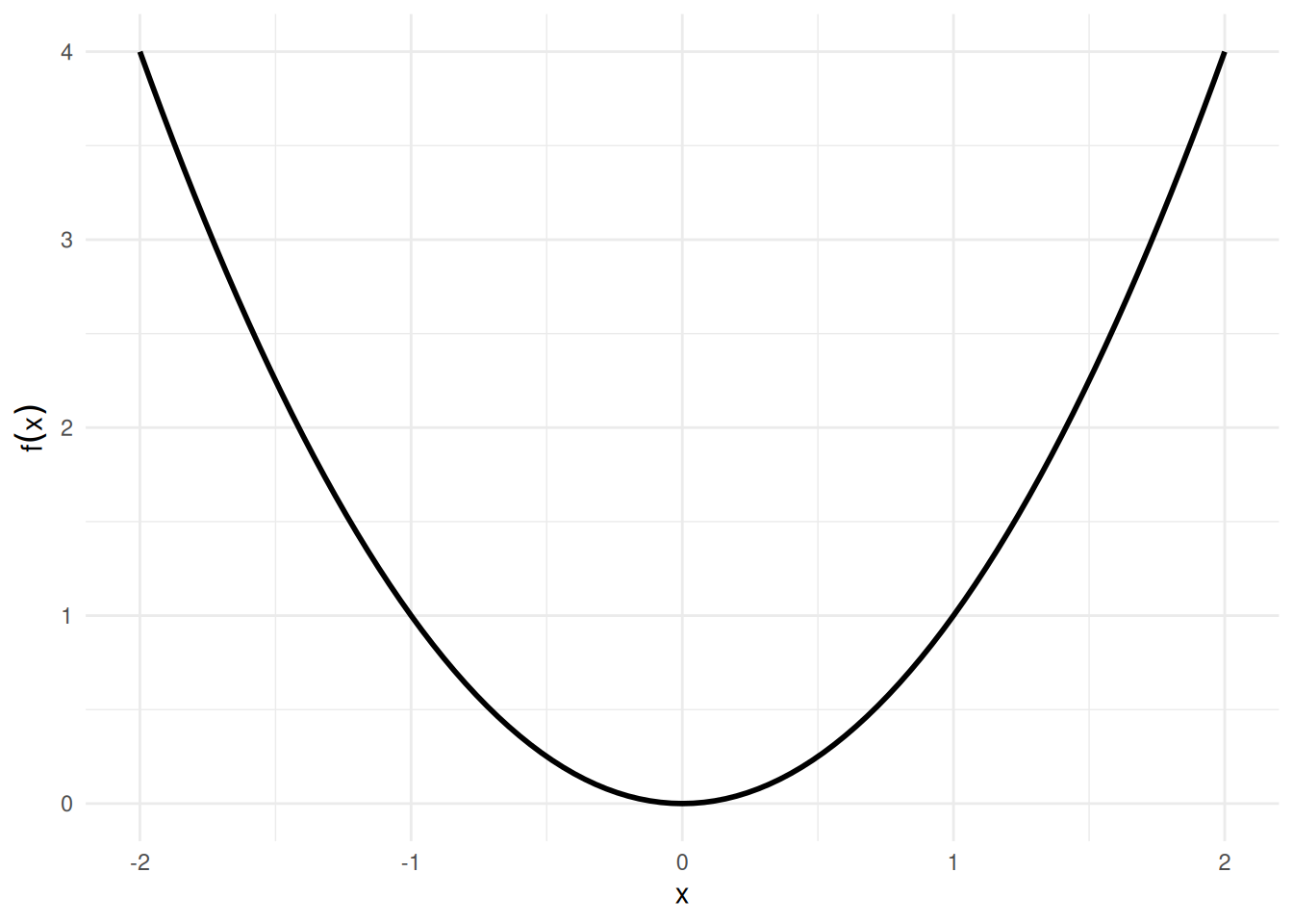
Example 3 (Antiderivative of a power function) For \(f(x) = x^2\), an antiderivative is \(F(x) = \frac{x^3}{3}\), since \(\frac{\partial}{\partial x}\frac{x^3}{3} = x^2 = f(x)\).
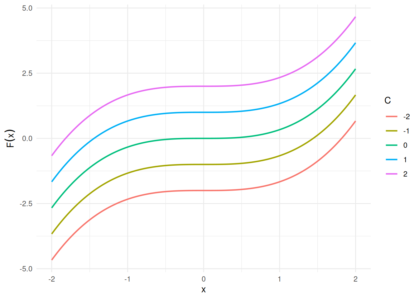
Adding any constant \(C\) gives another antiderivative; for example, with \(C = 7\), \(F(x) = \frac{x^3}{3} + 7\) also satisfies \(F'(x) = x^2\), since adding a constant does not change the derivative. See Figure 3.
[R code]
[R code]
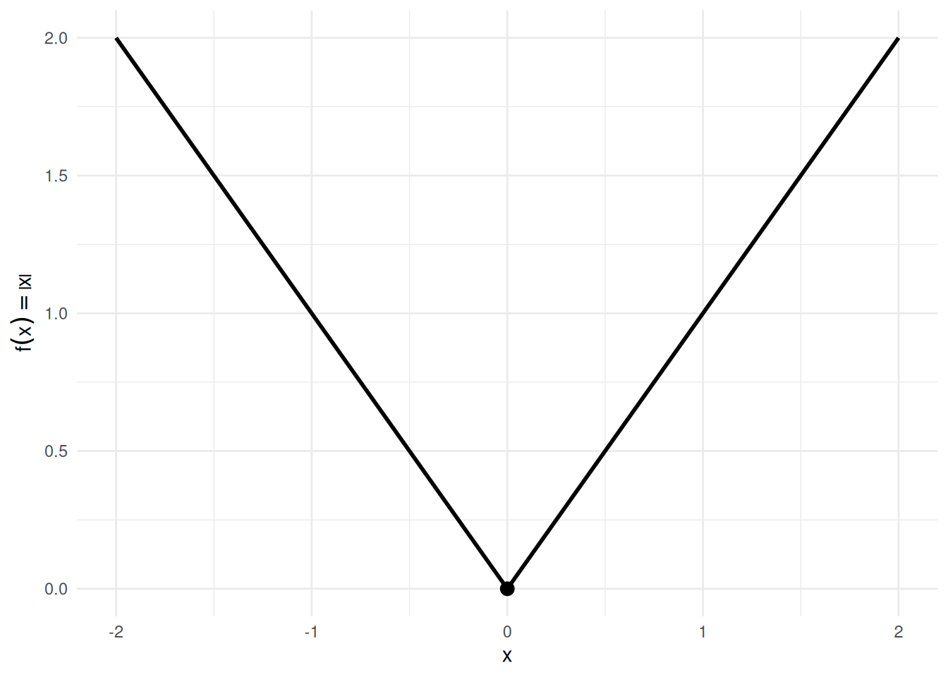
Example 6 (Continuous but not differentiable: \(\mathopen{}\left|x\right|\mathclose{}\)) The absolute-value function \(f(x) = \mathopen{}\left|x\right|\mathclose{}\) is continuous at \(x = 0\) (\(\lim_{x \to 0}\mathopen{}\left|x\right|\mathclose{} = 0 = \mathopen{}\left|0\right|\mathclose{}\)), but it is not differentiable at \(x = 0\): the left-derivative is \(-1\) and the right-derivative is \(+1\).
This shows that the converse of Theorem 30 fails: continuity does not imply differentiability. See Figure 4.
[R code]
Example 8 (Integrable but not continuous: a step function) Let \(f(x) = 0\) for \(x < \tfrac{1}{2}\) and \(f(x) = 1\) for \(x \ge \tfrac{1}{2}\). Then \(f\) is discontinuous at \(x = \tfrac{1}{2}\), but it is integrable on \([0, 1]\):
\[ \int_0^1 f(x)\,dx = \int_0^{1/2} 0\,dx + \int_{1/2}^1 1\,dx = 0 + \tfrac{1}{2} = \tfrac{1}{2}. \]
This shows that the converse of Theorem 31 fails: integrability does not imply continuity. See Figure 5.
[R code]
step_df <- data.frame(
x = c(0, 0.5, 0.5, 1),
y = c(0, 0, 1, 1),
segment = c("left", "left", "right", "right")
)
ggplot() +
geom_rect(
aes(xmin = 0.5, xmax = 1, ymin = 0, ymax = 1),
fill = "steelblue", alpha = 0.3
) +
geom_line(
data = step_df,
aes(x = x, y = y, group = segment),
linewidth = 1
) +
geom_point(aes(x = 0.5, y = 0), shape = 1, size = 3) +
geom_point(aes(x = 0.5, y = 1), shape = 16, size = 3) +
scale_x_continuous(breaks = c(0, 0.5, 1), labels = c("0", "1/2", "1")) +
scale_y_continuous(limits = c(-0.1, 1.2)) +
labs(x = "x", y = "f(x)") +
theme_minimal()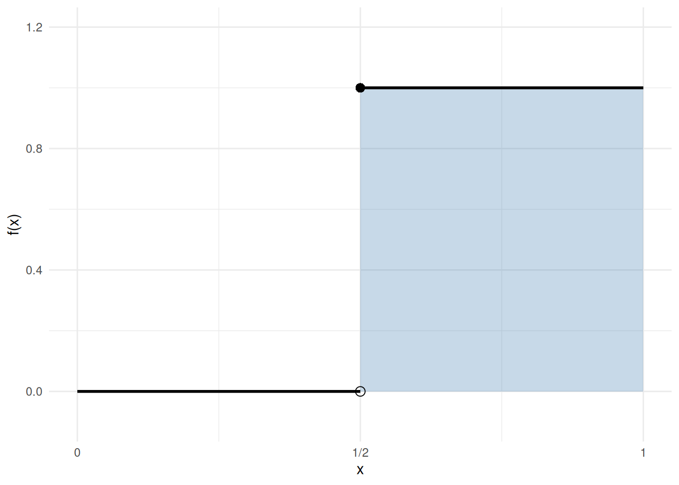
Example 9 (FTC Part 1 visualized: accumulation function for \(f(t) = 2t\)) Take \(f(t) = 2t\) on \([0, 2]\). The accumulation function from \(0\) is
\[F(x) \;\stackrel{\text{def}}{=}\; \int_0^x 2t\,dt \;=\; \mathopen{}\left[t^2\right]\mathclose{}_{t=0}^{t=x} \;=\; x^2 - 0^2 \;=\; x^2,\]
so \(F(x) = x^2\), and indeed \(F'(x) = 2x = f(x)\), as Theorem 32 Part 1 predicts. Figure 6 shows the integrand on the left (shaded area equals \(F(x)\) at each \(x\)) and the accumulation function \(F(x) = x^2\) on the right (its slope at \(x\) equals \(f(x) = 2x\)).
[R code]
ggplot() +
geom_area(
data = data.frame(t = seq(0, x_focus, length.out = 200)),
aes(x = t, y = 2 * t),
fill = "steelblue", alpha = 0.4
) +
geom_function(fun = \(t) 2 * t, xlim = c(0, 2.2), linewidth = 1) +
geom_vline(
data = data.frame(x = x_marks),
aes(xintercept = x, color = factor(x)),
linetype = "dashed", linewidth = 0.6
) +
labs(x = "t", y = "f(t) = 2t", color = "x") +
theme_minimal() +
theme(legend.position = "bottom")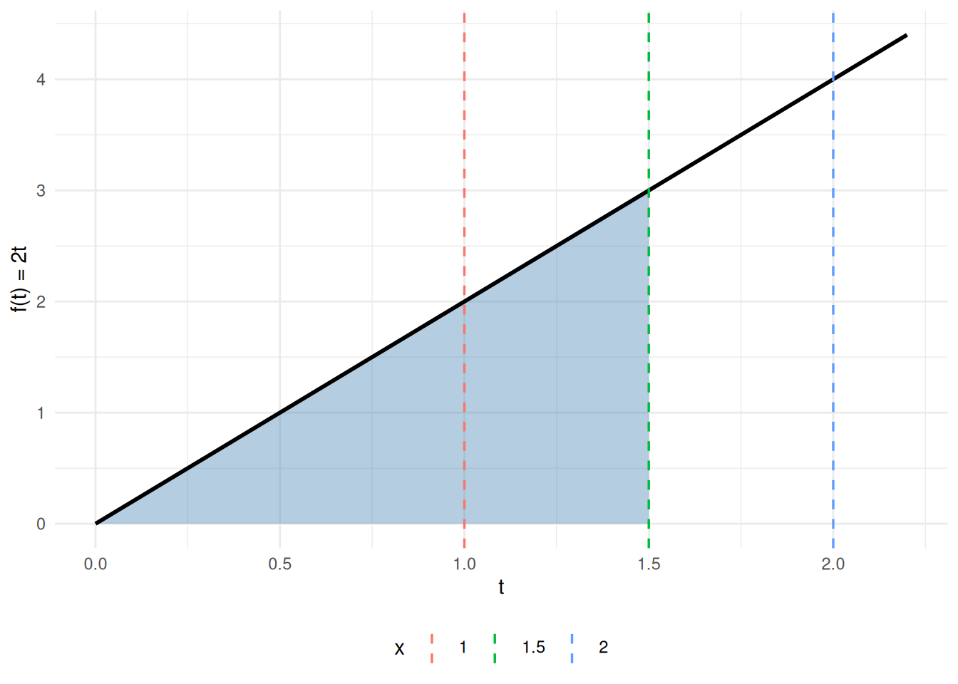
[R code]
slope_df <- data.frame(
x = x_marks,
Fx = x_marks^2,
slope = 2 * x_marks
)
ggplot() +
geom_function(fun = \(x) x^2, xlim = c(0, 2.2), linewidth = 1) +
geom_point(
data = slope_df,
aes(x = x, y = Fx, color = factor(x)),
size = 3
) +
geom_segment(
data = slope_df,
aes(
x = x - 0.3, xend = x + 0.3,
y = Fx - 0.3 * slope, yend = Fx + 0.3 * slope,
color = factor(x)
),
linewidth = 0.8
) +
labs(x = "x", y = expression(F(x) == x^2), color = "x") +
theme_minimal() +
theme(legend.position = "bottom")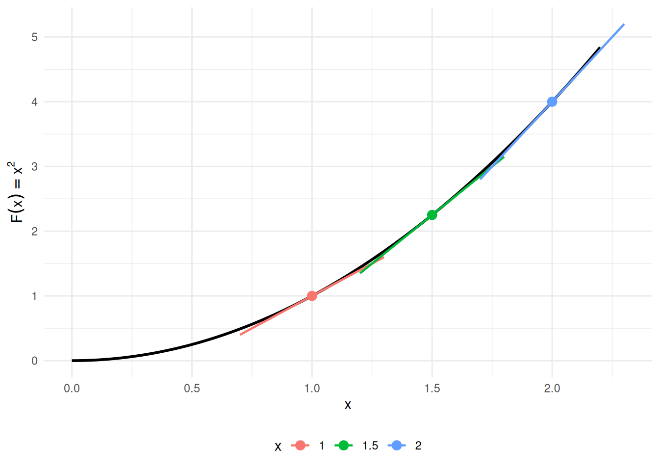
Example 10 (CDF and PDF of the exponential distribution) In what follows, \(f\) denotes the PDF and \(F\) the CDF — the same letters as the antiderivative pair in Definition 7, because the FTC will show \(F\) is exactly an antiderivative of \(f\).
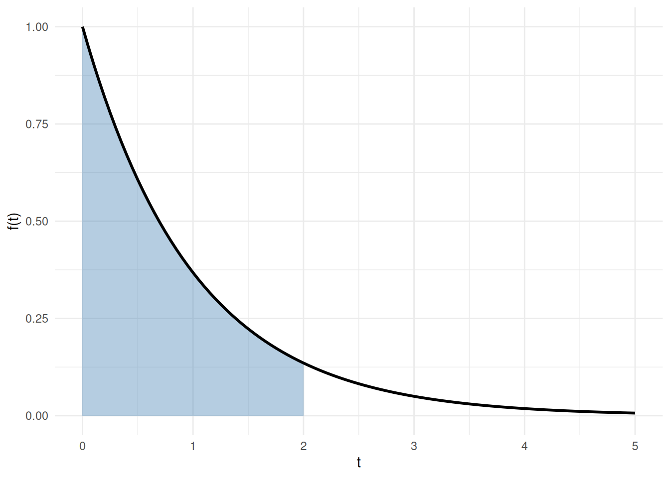
For the exponential distribution with rate parameter \(\lambda > 0\), the probability density function (PDF) is (Kleinbaum and Klein 2012, sec. II, p. 295, “Survival and Hazard Functions for Selected Distributions”):
\[f(t) = \lambda \text{e}^{-\lambda t}, \quad t \ge 0\]
FTC Part 2 gives the cumulative distribution function (CDF) from the PDF. Apply the \(\text{e}^{cx}\) rule from Theorem 28 with \(c = -\lambda\) to antidifferentiate the integrand:
\[ \begin{aligned} F(t) &= \int_0^t \lambda \text{e}^{-\lambda u}\,du \\ &= \mathopen{}\left[\lambda \cdot\frac{1}{-\lambda}\text{e}^{-\lambda u}\right]\mathclose{}_{u=0}^{u=t} \\ &= \mathopen{}\left[(-1)\text{e}^{-\lambda u}\right]\mathclose{}_{u=0}^{u=t} \\ &= \mathopen{}\left[-\text{e}^{-\lambda u}\right]\mathclose{}_{u=0}^{u=t} \\ &= -\text{e}^{-\lambda t} - \mathopen{}\left(-\text{e}^{0}\right)\mathclose{} \\ &= -\text{e}^{-\lambda t} - (-1) \\ &= 1 - \text{e}^{-\lambda t} \end{aligned} \]
FTC Part 1 recovers the PDF from the CDF:
\[ \begin{aligned} \frac{\partial}{\partial t} F(t) &= \frac{\partial}{\partial t}\mathopen{}\left(1 - \text{e}^{-\lambda t}\right)\mathclose{} \\ &= 0 - (-\lambda)\text{e}^{-\lambda t} \\ &= \lambda\text{e}^{-\lambda t} \\ &= f(t) \end{aligned} \]
For a concrete instance: with \(\lambda = 1\) (standard exponential), the probability that \(T \le 2\) is:
\[ F(2) = 1 - \text{e}^{-1 \cdot 2} = 1 - \text{e}^{-2} \approx 1 - 0.135 = 0.865 \]
See Figure 7.
[R code]
[R code]
ggplot() +
geom_function(
fun = \(t) 1 - exp(-lambda * t),
xlim = c(0, t_max), linewidth = 1
) +
geom_point(
aes(x = t_focus, y = F_at_focus),
size = 3, color = "steelblue"
) +
geom_segment(
aes(x = t_focus, xend = t_focus, y = 0, yend = F_at_focus),
linetype = "dashed", color = "steelblue"
) +
geom_segment(
aes(x = 0, xend = t_focus, y = F_at_focus, yend = F_at_focus),
linetype = "dashed", color = "steelblue"
) +
labs(x = "t", y = "F(t)") +
theme_minimal()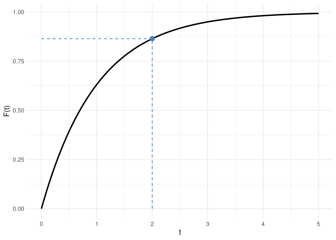
Example 11 (Changing the order of integration for a non-rectangular region) Adapted from (Larson and Edwards 2018, sec. 14.2, Example 4, pp. 984–985).
Let \(X\) and \(Y\) be independent \(\operatorname{Uniform}(0, 1)\) random variables, with joint density \(f(x, y) = 1\) on the unit square \([0, 1]^2\). Define the function \(g(x, y) = \text{e}^{-x^2}\,\mathbb{1}\mathopen{}\left(y \le x\right)\mathclose{}\), and compute its expectation \(\operatorname{E}\mathopen{}\left[g(X, Y)\right]\mathclose{}\).
Because the joint density equals \(1\) on \([0, 1]^2\), this expectation is the double integral of \(g\) over the unit square:
\[\operatorname{E}\mathopen{}\left[g(X, Y)\right]\mathclose{} = \iint_{[0, 1]^2} g(x, y)\,dA.\]
The indicator factor \(\mathbb{1}\mathopen{}\left(y \le x\right)\mathclose{}\) equals \(1\) on the triangular region where \(y \le x\) and \(0\) elsewhere, so only that region, namely \(D = \{(x, y) : x \in [0, 1],\; y \in [0, x]\}\) (Figure 8), contributes, and there \(g(x, y) = \text{e}^{-x^2}\):
\[\operatorname{E}\mathopen{}\left[g(X, Y)\right]\mathclose{} = \iint_D \text{e}^{-x^2}\,dA.\]
[R code]
region <- data.frame(x = c(0, 1, 1), y = c(0, 0, 1))
ggplot2::ggplot(region, ggplot2::aes(x = x, y = y)) +
ggplot2::geom_polygon(
fill = "steelblue", alpha = 0.4, color = "black", linewidth = 0.7
) +
ggplot2::annotate(
"text", x = 0.65, y = 0.28, label = "D", size = 8, fontface = "italic"
) +
ggplot2::annotate(
"text", x = 0.36, y = 0.52, label = "y == x",
parse = TRUE, angle = 45
) +
ggplot2::annotate(
"text", x = 1.08, y = 0.5, label = "x == 1",
parse = TRUE, angle = 90, hjust = 0.5
) +
ggplot2::annotate(
"text", x = 0.5, y = -0.1, label = "y == 0", parse = TRUE
) +
ggplot2::scale_x_continuous(breaks = c(0, 0.5, 1), limits = c(-0.1, 1.3)) +
ggplot2::scale_y_continuous(breaks = c(0, 0.5, 1), limits = c(-0.2, 1.2)) +
ggplot2::coord_equal() +
ggplot2::labs(x = "x", y = "y") +
ggplot2::theme_minimal()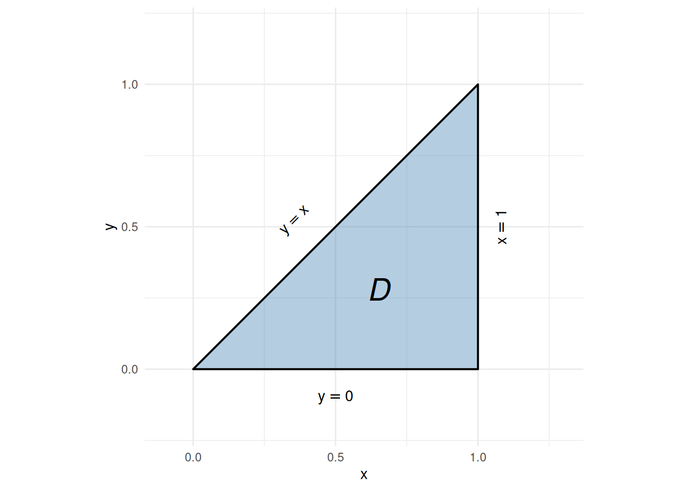
Order \(dx\,dy\) is intractable. Re-describing \(D\) as \(D = \{(x, y) : y \in [0, 1],\; x \in [y, 1]\}\), the inner integral is
\[\int_y^1 \text{e}^{-x^2}\,dx,\]
which has no elementary antiderivative.
Order \(dy\,dx\) works. Applying Theorem 33 Part 1 (\(\text{e}^{-x^2}\) is continuous and \(D\) is the vertically simple region \(x \in [0, 1]\), \(y \in [0, x]\)):
\[ \begin{aligned} \iint_D \text{e}^{-x^2}\,dA &= \int_0^1\!\int_0^x \text{e}^{-x^2}\,dy\,dx \\&= \int_0^1 \text{e}^{-x^2}\mathopen{}\left(\int_0^x dy\right)\mathclose{}\,dx \\&= \int_0^1 x\,\text{e}^{-x^2}\,dx \\&= \mathopen{}\left[-\frac{1}{2}\,\text{e}^{-x^2}\right]\mathclose{}_0^1 \\&= -\frac{1}{2}\mathopen{}\left(\text{e}^{-1} - 1\right)\mathclose{} \\&= \frac{e - 1}{2e} \\&\approx 0.316 \end{aligned} \]
The solid whose volume equals this integral is shown in Figure 9.
[R code]
n_grid <- 51
x_seq <- seq(0, 1, length.out = n_grid)
y_seq <- seq(0, 1, length.out = n_grid)
z_mat <- outer(x_seq, y_seq, function(x, y) {
z <- exp(-x^2)
z[y > x] <- NA
z
})
plotly::plot_ly(x = ~x_seq, y = ~y_seq, z = ~t(z_mat)) |>
plotly::add_surface(showscale = FALSE) |>
plotly::layout(scene = list(
xaxis = list(title = "x"),
yaxis = list(title = "y"),
zaxis = list(title = "z = exp(-x^2)"),
camera = list(eye = list(x = 1.6, y = -1.6, z = 0.8))
))Example 13 (Evaluating a double integral on a rectangle) Structure adapted from (Larson and Edwards 2018, sec. 14.2, Example 2, pp. 982–983); the integrand \(x^2 + y^2\) is original, chosen so the integral equals \(\operatorname{E}\mathopen{}\left[g(X, Y)\right]\mathclose{}\) for \(g(x, y) = x^2 + y^2\).
Let \(X\) and \(Y\) be independent \(\operatorname{Uniform}(0, 1)\) random variables, with joint density \(f(x, y) = 1\) on the unit square \(R = \{(x, y) : x \in [0, 1],\; y \in [0, 1]\}\) (Figure 11). Define the function \(g(x, y) = x^2 + y^2\), and compute its expectation \(\operatorname{E}\mathopen{}\left[g(X, Y)\right]\mathclose{}\).
Because the joint density equals \(1\) on \(R\), this expectation is the double integral of \(g\) over \(R\):
\[\operatorname{E}\mathopen{}\left[g(X, Y)\right]\mathclose{} = \iint_R \mathopen{}\left(x^2 + y^2\right)\mathclose{}\,dA.\]
[R code]
ggplot2::ggplot() +
ggplot2::annotate(
"rect", xmin = 0, xmax = 1, ymin = 0, ymax = 1,
fill = "steelblue", alpha = 0.4, color = "black", linewidth = 0.7
) +
ggplot2::annotate(
"text", x = 0.5, y = 0.5, label = "R", size = 8, fontface = "italic"
) +
ggplot2::scale_x_continuous(breaks = c(0, 1), limits = c(-0.15, 1.25)) +
ggplot2::scale_y_continuous(breaks = c(0, 1), limits = c(-0.15, 1.25)) +
ggplot2::coord_equal() +
ggplot2::labs(x = "x", y = "y") +
ggplot2::theme_minimal()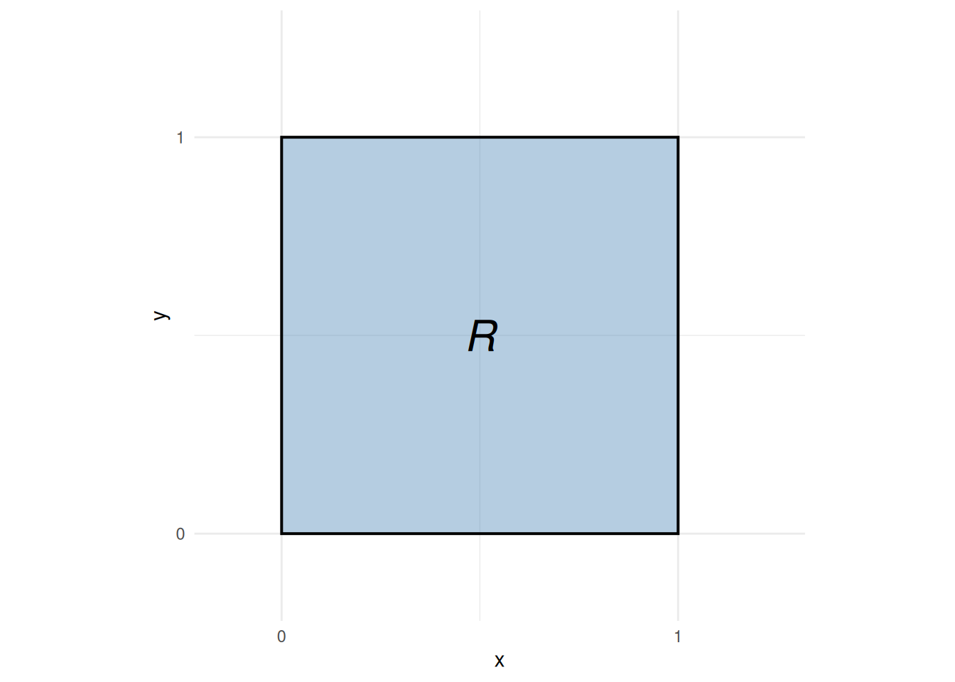
The integrand is continuous on \(R\), so Corollary 5 applies and either order of integration yields the same value.
Integrating \(y\) first, then \(x\):
\[ \begin{aligned} \operatorname{E}\mathopen{}\left[g(X, Y)\right]\mathclose{} &= \int_0^1\!\int_0^1 \mathopen{}\left(x^2 + y^2\right)\mathclose{}\,dy\,dx \\&= \int_0^1 \mathopen{}\left[x^2 y + \frac{y^3}{3}\right]\mathclose{}_0^1\,dx \\&= \int_0^1 \mathopen{}\left(x^2 + \frac{1}{3}\right)\mathclose{}\,dx \\&= \mathopen{}\left[\frac{x^3}{3} + \frac{x}{3}\right]\mathclose{}_0^1 \\&= \frac{2}{3} \end{aligned} \]
Integrating \(x\) first, then \(y\) (verifying the order can be swapped):
\[ \begin{aligned} \int_0^1\!\int_0^1 \mathopen{}\left(x^2 + y^2\right)\mathclose{}\,dx\,dy &= \int_0^1 \mathopen{}\left[\frac{x^3}{3} + y^2 x\right]\mathclose{}_0^1\,dy \\&= \int_0^1 \mathopen{}\left(\frac{1}{3} + y^2\right)\mathclose{}\,dy \\&= \mathopen{}\left[\frac{y}{3} + \frac{y^3}{3}\right]\mathclose{}_0^1 \\&= \frac{2}{3} \end{aligned} \]
Both orders give \(\frac{2}{3}\), as Corollary 5 guarantees.
As a cross-check, linearity of expectation gives the same value: since \(\operatorname{E}\mathopen{}\left[X^2\right]\mathclose{} = \int_0^1 x^2\,dx = \frac{1}{3}\) for \(X \sim \operatorname{Uniform}(0, 1)\) (and likewise for \(Y\)),
\[\operatorname{E}\mathopen{}\left[g(X, Y)\right]\mathclose{} = \operatorname{E}\mathopen{}\left[X^2 + Y^2\right]\mathclose{} = \operatorname{E}\mathopen{}\left[X^2\right]\mathclose{} + \operatorname{E}\mathopen{}\left[Y^2\right]\mathclose{} = \frac{1}{3} + \frac{1}{3} = \frac{2}{3}.\]
The solid whose volume equals this integral is shown in Figure 12.
[R code]
n_grid <- 41
x_seq <- seq(0, 1, length.out = n_grid)
y_seq <- seq(0, 1, length.out = n_grid)
z_mat <- outer(x_seq, y_seq, function(x, y) x^2 + y^2)
plotly::plot_ly(x = ~x_seq, y = ~y_seq, z = ~t(z_mat)) |>
plotly::add_surface(showscale = FALSE) |>
plotly::layout(scene = list(
xaxis = list(title = "x"),
yaxis = list(title = "y"),
zaxis = list(title = "z", range = c(0, 2))
))